Week 2 – Introduction to R data structures
Aims
- To demonstrate the R data structures
Data structures in R
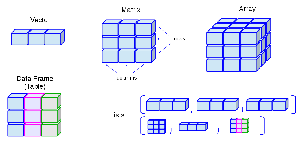
- R has many data structures. These include
Matrices
- In R matrices are an extension of the numeric or character vectors.
- As with atomic vectors, the elements of a matrix must be of the same data type.
- The matrix can be viewed as a collection of vectors
- Matrix rows and columns are vectors
- All the vectors hold identical data type
- The vectors must have the same length
x <- c(1:9)
is.vector(x)
## [1] TRUEtypeof(x)## [1] "integer"y <- matrix(data=1:9, nrow = 3, ncol = 3) # create a matrix
class(y)## [1] "matrix" "array"typeof(y)## [1] "integer"- In contrast to vectors, matrices and data frames are two dimensional
data structures
- First dimension: rows
- Second dimension: columns
- dim(): Provides the dimensions of an object
- nrow(): gives number of rows
- ncol(): gives number of columns
dim(y) # get dimensions of an object## [1] 3 3nrow(y) # gives number of rows## [1] 3ncol(y) # gives number of columns## [1] 3- Unlike vectors, sub-setting requires both rows and columns to be provided
- Like vector subscript operator “[]” is used to access the values
- Unlike vector, matrix is a two dimensional data structure
- general syntax: matrix[ rows , columns ]
y[] # gives all the values in a matrix## [,1] [,2] [,3]
## [1,] 1 4 7
## [2,] 2 5 8
## [3,] 3 6 9y[1,2] # get the value from 1st row and 2 columns## [1] 4y[1,] # get all the values from 1st row## [1] 1 4 7y[,3] # get all the values from 3rd column## [1] 7 8 9y[c(1,3), c(2,3)] # get 1st and 3rd values from 2nd and 3rd column## [,1] [,2]
## [1,] 4 7
## [2,] 6 9- Like vector matrix can hold only one type of data, if we try to mix two are more different data type, R implicitly convert into one type
typeof(y)## [1] "integer"y## [,1] [,2] [,3]
## [1,] 1 4 7
## [2,] 2 5 8
## [3,] 3 6 9y[2,3]## [1] 8y[2,3] <- "A" # replace
y## [,1] [,2] [,3]
## [1,] "1" "4" "7"
## [2,] "2" "5" "A"
## [3,] "3" "6" "9"typeof(y)## [1] "character"Lists
- R’s simplest structure that combines data of different types is a list.
- A list is a collection of any data structures
- List can be of different types and different lengths.
- A list can be a collection of lists.
- Lists are very flexible data structures that can hold anything.
my_first_list <- list(1:10, c("a", "b", "c"),
                      c(TRUE, FALSE), 100,
                      c(1.3, 2.2, 0.75, 3.8))
my_first_list
## [[1]]
## [1] 1 2 3 4 5 6 7 8 9 10
##
## [[2]]
## [1] "a" "b" "c"
##
## [[3]]
## [1] TRUE FALSE
##
## [[4]]
## [1] 100
##
## [[5]]
## [1] 1.30 2.20 0.75 3.80my_first_list has five elements and when printed out like this looks quite strange at first sight. Note how each of the elements of a list is referred to by an index within 2 sets of square brackets or one set of square. This gives a clue to how you can access individual elements in the list.
- How to access the elements from the list?
- Using any one of the following three operator …
- “[]”: Standard subscript operator, works like in a vector. The output is still a list.
- “[[]]”: This operator can only take one index number at a time and the output will be the data structure for that element.
- “$”: to extract an element from a list or a column from a data frame by name.
- Using any one of the following three operator …
length(my_first_list)## [1] 5my_first_list[1] # get element one from the list## [[1]]
## [1] 1 2 3 4 5 6 7 8 9 10my_first_list[1:3] # get element one from the list## [[1]]
## [1] 1 2 3 4 5 6 7 8 9 10
##
## [[2]]
## [1] "a" "b" "c"
##
## [[3]]
## [1] TRUE FALSElength(my_first_list)## [1] 5my_first_list[[1]] # get element one from the list## [1] 1 2 3 4 5 6 7 8 9 10my_first_list[[5]] # get element one from the list## [1] 1.30 2.20 0.75 3.80- Elements in lists are normally named
named_list <- list(
  city_name=c("Cambridge", "London", "Oxford"),
  population=c(1.62, 8.9, 1.5 ) )

named_list
## $city_name
## [1] "Cambridge" "London" "Oxford"
##
## $population
## [1] 1.62 8.90 1.50named_list$city_name # equivalent to named_list[[1]]## [1] "Cambridge" "London" "Oxford"named_list$population # equivalent to named_list[[2]]## [1] 1.62 8.90 1.50- You can modify lists either by adding addition elements or modifying existing ones.
named_list$city_name[2] <- "LONDON"
named_list
## $city_name
## [1] "Cambridge" "LONDON" "Oxford"
##
## $population
## [1] 1.62 8.90 1.50Lists can be thought of as a ragbag collection of things without a very clear structure. You probably won’t find yourself creating list objects of the kind we’ve seen above when analyzing your own data. However, the list provides the basic underlying structure to the data frame that we’ll be using throughout the rest of this course.
The other area where you’ll come across lists is as the return value for many of the statistical tests and procedures such as linear regression that you can carry out in R.
To demonstrate, we’ll run a t-test comparing two sets of samples drawn from subtly different normal distributions. We’ve already come across the rnorm() function for creating random numbers based on a normal distribution.
sample_1 <- rnorm(n = 100, mean=5, sd=1)
sample_2 <- rnorm(n = 100, mean=7, sd=1)

result <- t.test(x=sample_1, y=sample_2)

is.list(result) # test if object is a list
## [1] TRUEresult##
## Welch Two Sample t-test
##
## data: sample_1 and sample_2
## t = -14.422, df = 196.42, p-value < 2.2e-16
## alternative hypothesis: true difference in means is not equal to 0
## 95 percent confidence interval:
## -2.179627 -1.655238
## sample estimates:
## mean of x mean of y
## 5.064695 6.982128names(result) # list names of the object## [1] "statistic" "parameter" "p.value" "conf.int" "estimate"
## [6] "null.value" "stderr" "alternative" "method" "data.name"result$statistic## t
## -14.42213result$p.value## [1] 1.242028e-32Data frames
- A much more useful data structure and the one we will mostly be using for the rest of the course is the data frame.
- This is actually a special type of list in which all the elements are vectors of the same length.
df <- data.frame(
  city_name=c("Cambridge", "London", "Oxford"),
  population=c(1.62, 8.9, 1.5 ))
df
## city_name population
## 1 Cambridge 1.62
## 2 London 8.90
## 3 Oxford 1.50class(df)## [1] "data.frame"dim(df)## [1] 3 2- R provides many built-in data sets, most of which are represented as data frames.
- data(): lists all the avilable built-in data sets
- One popular data set is
iris - To know more about any data set, one can use
help()or?to get help - iris:
- data frame with 150 observations (rows)
- 5 variables (columns)
- Sepal.Length
- Sepal.Width
- Petal.Length
- Petal.Width
- Species
- data frame with 150 observations (rows)
- To bring one of these internal data sets to the fore, you can just start using it by name.
head(iris)## Sepal.Length Sepal.Width Petal.Length Petal.Width Species
## 1 5.1 3.5 1.4 0.2 setosa
## 2 4.9 3.0 1.4 0.2 setosa
## 3 4.7 3.2 1.3 0.2 setosa
## 4 4.6 3.1 1.5 0.2 setosa
## 5 5.0 3.6 1.4 0.2 setosa
## 6 5.4 3.9 1.7 0.4 setosa- You can also get help for a data set such as iris in the usual way.
?iris # get help for iris dataThis reveals that iris is a rather famous old data set of measurements taken by the esteemed British statistician and geneticist, Ronald Fisher (he of Fisher’s exact test fame).
A data frame is a special type of list so you can access its columns in the same way as we saw previously for lists.
names(iris)## [1] "Sepal.Length" "Sepal.Width" "Petal.Length" "Petal.Width" "Species"iris$Petal.Width # or equivalently iris[["Petal.Width"]] or iris[[4]]## [1] 0.2 0.2 0.2 0.2 0.2 0.4 0.3 0.2 0.2 0.1 0.2 0.2 0.1 0.1 0.2 0.4 0.4 0.3
## [19] 0.3 0.3 0.2 0.4 0.2 0.5 0.2 0.2 0.4 0.2 0.2 0.2 0.2 0.4 0.1 0.2 0.2 0.2
## [37] 0.2 0.1 0.2 0.2 0.3 0.3 0.2 0.6 0.4 0.3 0.2 0.2 0.2 0.2 1.4 1.5 1.5 1.3
## [55] 1.5 1.3 1.6 1.0 1.3 1.4 1.0 1.5 1.0 1.4 1.3 1.4 1.5 1.0 1.5 1.1 1.8 1.3
## [73] 1.5 1.2 1.3 1.4 1.4 1.7 1.5 1.0 1.1 1.0 1.2 1.6 1.5 1.6 1.5 1.3 1.3 1.3
## [91] 1.2 1.4 1.2 1.0 1.3 1.2 1.3 1.3 1.1 1.3 2.5 1.9 2.1 1.8 2.2 2.1 1.7 1.8
## [109] 1.8 2.5 2.0 1.9 2.1 2.0 2.4 2.3 1.8 2.2 2.3 1.5 2.3 2.0 2.0 1.8 2.1 1.8
## [127] 1.8 1.8 2.1 1.6 1.9 2.0 2.2 1.5 1.4 2.3 2.4 1.8 1.8 2.1 2.4 2.3 1.9 2.3
## [145] 2.5 2.3 1.9 2.0 2.3 1.8- Viewing data frames is made easier with these functions
- head(): Shows first 6 lines of a data frame
- tail(): Shows first 6 lines of a data frame
- View(): Shows data frame in excel like format
head(iris)## Sepal.Length Sepal.Width Petal.Length Petal.Width Species
## 1 5.1 3.5 1.4 0.2 setosa
## 2 4.9 3.0 1.4 0.2 setosa
## 3 4.7 3.2 1.3 0.2 setosa
## 4 4.6 3.1 1.5 0.2 setosa
## 5 5.0 3.6 1.4 0.2 setosa
## 6 5.4 3.9 1.7 0.4 setosatail(iris)## Sepal.Length Sepal.Width Petal.Length Petal.Width Species
## 145 6.7 3.3 5.7 2.5 virginica
## 146 6.7 3.0 5.2 2.3 virginica
## 147 6.3 2.5 5.0 1.9 virginica
## 148 6.5 3.0 5.2 2.0 virginica
## 149 6.2 3.4 5.4 2.3 virginica
## 150 5.9 3.0 5.1 1.8 virginicaView(iris)- In that last example we extracted the Petal.Width column which itself is a vector. We can further subset the values in that column to, say, return the first 10 values only.
iris$Petal.Length[1:10]## [1] 1.4 1.4 1.3 1.5 1.4 1.7 1.4 1.5 1.4 1.5- Matrix-like syntax can be used to access both rows and columns.
- df[ row index, column index]
# df[ row index, column index]
iris[ 1:4, 1:3] # rows from 1 to 4 and columns from 1 to 3
## Sepal.Length Sepal.Width Petal.Length
## 1 5.1 3.5 1.4
## 2 4.9 3.0 1.4
## 3 4.7 3.2 1.3
## 4 4.6 3.1 1.5iris[c(1,4,7), c(2,4)] # rows from1,4 and 7 and columns from 2 and 4## Sepal.Width Petal.Width
## 1 3.5 0.2
## 4 3.1 0.2
## 7 3.4 0.3- To extract values from a data frame, row/column names may also be used
iris[c(1,4,7), c("Sepal.Width","Species" )] # iris[c(1,4,7), c(2,5)] ## Sepal.Width Species
## 1 3.5 setosa
## 4 3.1 setosa
## 7 3.4 setosa- We can also use conditional sub-setting to extract the rows that meet certain conditions, e.g. all the rows with Sepal.Length of 5.
iris[iris$Sepal.Length == 5, ]## Sepal.Length Sepal.Width Petal.Length Petal.Width Species
## 5 5 3.6 1.4 0.2 setosa
## 8 5 3.4 1.5 0.2 setosa
## 26 5 3.0 1.6 0.2 setosa
## 27 5 3.4 1.6 0.4 setosa
## 36 5 3.2 1.2 0.2 setosa
## 41 5 3.5 1.3 0.3 setosa
## 44 5 3.5 1.6 0.6 setosa
## 50 5 3.3 1.4 0.2 setosa
## 61 5 2.0 3.5 1.0 versicolor
## 94 5 2.3 3.3 1.0 versicolor- One can use & (and), | (or) and ! (not) logical operators for complex sub-setting.
iris[iris$Sepal.Length == 5 & iris$Species == "setosa", ]## Sepal.Length Sepal.Width Petal.Length Petal.Width Species
## 5 5 3.6 1.4 0.2 setosa
## 8 5 3.4 1.5 0.2 setosa
## 26 5 3.0 1.6 0.2 setosa
## 27 5 3.4 1.6 0.4 setosa
## 36 5 3.2 1.2 0.2 setosa
## 41 5 3.5 1.3 0.3 setosa
## 44 5 3.5 1.6 0.6 setosa
## 50 5 3.3 1.4 0.2 setosaA data frame is the most common data structure you will encounter as
a beginner. As you can see from the examples above, the syntax is tricky
and not intuitive at all. In order to overcome this problem, R has a
package called tidyverse. The
tidyverse package combines eight other packages into one. Two important
packages in tidyverse are dplyr and
ggplot2
- dplyr: Makes working with data frames fun and easy
- ggplot2: Creates beautiful plots with ease.
From next week you will be working with tidyverse.
summary()is a very useful function that summarises each column in a data frame
summary(iris)## Sepal.Length Sepal.Width Petal.Length Petal.Width
## Min. :4.300 Min. :2.000 Min. :1.000 Min. :0.100
## 1st Qu.:5.100 1st Qu.:2.800 1st Qu.:1.600 1st Qu.:0.300
## Median :5.800 Median :3.000 Median :4.350 Median :1.300
## Mean :5.843 Mean :3.057 Mean :3.758 Mean :1.199
## 3rd Qu.:6.400 3rd Qu.:3.300 3rd Qu.:5.100 3rd Qu.:1.800
## Max. :7.900 Max. :4.400 Max. :6.900 Max. :2.500
## Species
## setosa :50
## versicolor:50
## virginica :50
##
##
## Data Type Checking and Conversion: is vs
as
“is” family functions
Is function start with “is.” like is.vector(), is.character()
Output of is family of functions is a logical value TRUE or FALSE
- What type of data does the object contain?
- typeof(): Indicates the type of data contained in the object
- is.character(): to test if the object holds character type data
- is.double(): to test if the object holds decimal type data
- is.numeric(): to test if the object holds numeric type data
- is.integer(): to test if the object holds integer type data
- is.logical(): to test if the object holds logical type data
- What type of data structure does the object represent?
- class(): Describes the type of data structure that the object represents
- is.vector(): To determine if the object is a vector
- is.factor(): To determine if the object is a factor
- is.matrix(): To determine if the object is a matrix
- is.data.frame(): To determine if the object is a data frame
- What type of data does the object contain?
x <- 1:100
typeof(x)
## [1] "integer"is.integer(x)## [1] TRUEis.vector(x)## [1] TRUEis.factor(x)## [1] FALSE“as” family functions
For converting one data type to another data type or one data structure to another data structure
As function start with “as.” like as.vector(), as.character()
- Convert one data type to another data type
- as.character(): convert to character type data
- as.numeric()
- as.integer()
- as.logical()
- Convert one type of data structure to another
- as.vector()
- as.matrix()
- as.factor()
- as.data.frame()
- Convert one data type to another data type
x <- 1:100
typeof(x)
## [1] "integer"y <- as.character(x)
typeof(y)## [1] "character"is.vector(x)## [1] TRUEz <- as.matrix(x)
is.matrix(z)## [1] TRUEExercises
Using
mtcarsdataset answer the following.- How many rows and columns in the
mtcarsdata set? - How many cars in the
mtcarsdata set have 8 cylinders? - How many cars in the
mtcarsdata set have 6 cylinders and more than 3 gears?
- How many rows and columns in the
Answer
# 1 a
nrow(mtcars)
## [1] 32ncol(mtcars)## [1] 11# 1 b
sum(mtcars$cyl == 8)## [1] 14# 1 c
sum(mtcars$cyl== 6 & mtcars$gear > 3)## [1] 5- Extract 3rd and 5th rows with 1st and 3rd columns from
mtcarsdata set.
Answer
mtcars[c(3,5), c(1,3)]## mpg disp
## Datsun 710 22.8 108
## Hornet Sportabout 18.7 360- From
airqualitydata set- Identify the data structure of the first row by extracting it?
- Identify the data structure of the first column by extracting it?
Answer
# 3 a
class(airquality[1,])
## [1] "data.frame"# 3 b
class(airquality[,1])## [1] "integer"is.vector(airquality[,1])## [1] TRUEis.data.frame(airquality[,1])## [1] FALSE- Using
airqualitydata set- Show first 10 rows
- Show last 2 rows
- list all the column names available
Answer
# 4 a
head(airquality, n=10)
## Ozone Solar.R Wind Temp Month Day
## 1 41 190 7.4 67 5 1
## 2 36 118 8.0 72 5 2
## 3 12 149 12.6 74 5 3
## 4 18 313 11.5 62 5 4
## 5 NA NA 14.3 56 5 5
## 6 28 NA 14.9 66 5 6
## 7 23 299 8.6 65 5 7
## 8 19 99 13.8 59 5 8
## 9 8 19 20.1 61 5 9
## 10 NA 194 8.6 69 5 10# 4 b
tail(airquality, n=2)## Ozone Solar.R Wind Temp Month Day
## 152 18 131 8.0 76 9 29
## 153 20 223 11.5 68 9 30# 4 c
names(airquality)## [1] "Ozone" "Solar.R" "Wind" "Temp" "Month" "Day"colnames(airquality)## [1] "Ozone" "Solar.R" "Wind" "Temp" "Month" "Day"- Using
airqualitydata set, can you test Ozone production and solar radiation are correlated and answer the following. Hint: Usecor.testfunction.- Get correlation coefficient confidence interval
- what is the p-value?
- What is the estimated correlation coefficient?
Answer
# 1 a
results <- cor.test(airquality$Ozone, airquality$Solar.R)
results$conf.int
## [1] 0.173194 0.502132
## attr(,"conf.level")
## [1] 0.95# 1 b
result$p.value## [1] 1.242028e-32# 1 c
results$estimate## cor
## 0.3483417