Week 4 – Data manipulation with dplyr
Learning objectives
- Learn the five key dplyr functions for manipulating your data
select()for selecting a subset of variables, i.e. selecting columns in your tablefilter()for selecting observations based on their values, i.e. selecting rows in your tablearrange()for sorting the observations in your tablemutate()for creating a new variable or modifying an existing variablesummarise()for collapsing values in one of more columns to a single summary value- Chain operations together into a workflow using pipes
- Learn about faceting in ggplot2 to split your data into separate categories and create a series of sub-plots arranged in a grid
Data manipulation with dplyr
dplyr is one of the packages that gets loaded as part of the tidyverse.
library(tidyverse)dplyr is the Swiss army knife in the tidyverse, providing many useful functions for manipulating tabular data in data frames or tibbles. We’re going to look at the key functions for filtering our data, modifying the contents and computing summary statistics.
We’ll also introduce the pipe operator, %>%, for chaining operations together into mini workflows in a way that makes for more readable and maintainable code.
Finally, we’ll return to plotting and look at a powerful feature of ggplot2, faceting, that allows you to divide your plots into subplots by splitting the observations based on one or more categorical variables.
We’ll again use the METABRIC data set to illustrate how these operations work.
metabric <- read_csv("data/metabric_clinical_and_expression_data.csv")
metabric
## # A tibble: 1,904 x 32
## Patient_ID Cohort Age_at_diagnosis Survival_time Survival_status
## <chr> <dbl> <dbl> <dbl> <chr>
## 1 MB-0000 1 75.6 140. LIVING
## 2 MB-0002 1 43.2 84.6 LIVING
## 3 MB-0005 1 48.9 164. DECEASED
## 4 MB-0006 1 47.7 165. LIVING
## 5 MB-0008 1 77.0 41.4 DECEASED
## 6 MB-0010 1 78.8 7.8 DECEASED
## 7 MB-0014 1 56.4 164. LIVING
## 8 MB-0022 1 89.1 99.5 DECEASED
## 9 MB-0028 1 86.4 36.6 DECEASED
## 10 MB-0035 1 84.2 36.3 DECEASED
## # … with 1,894 more rows, and 27 more variables: Vital_status <chr>,
## # Chemotherapy <chr>, Radiotherapy <chr>, Tumour_size <dbl>,
## # Tumour_stage <dbl>, Neoplasm_histologic_grade <dbl>,
## # Lymph_nodes_examined_positive <dbl>, Lymph_node_status <dbl>,
## # Cancer_type <chr>, ER_status <chr>, PR_status <chr>,
## # HER2_status <chr>, HER2_status_measured_by_SNP6 <chr>, PAM50 <chr>,
## # `3-gene_classifier` <chr>, Nottingham_prognostic_index <dbl>,
## # Cellularity <chr>, Integrative_cluster <chr>, Mutation_count <dbl>,
## # ESR1 <dbl>, ERBB2 <dbl>, PGR <dbl>, TP53 <dbl>, PIK3CA <dbl>,
## # GATA3 <dbl>, FOXA1 <dbl>, MLPH <dbl>Data semantics
We use the terms ‘observation’ and ‘variable’ a lot in this course. As a reminder from week 2, when we talk about an observation, we’re talking about a set of values measured for the same unit or thing, e.g. a person or a date, and when we talk about a variable we are really talking about the attribute that we are measuring or recording, e.g. height, temperature or expression value.
Observations are represented as rows in our data frames or tibbles, while the columns correspond to variables.
From “Tidy Data” by Hadley Wickham, The Journal of Statistical Software, vol. 59, 2014.
A data set is a collection of values, usually either numbers (if quantitative) or character strings (if qualitative). Values are organised in two ways. Every value belongs to a variable and an observation.
A variable contains all values that measure the same underlying attribute (like height, temperature, duration) across units.
An observation contains all values measured on the same unit (like a person or a day) across attributes.
dplyr verbs
We will be looking at the 5 key dplyr functions this week:
filter()for filtering rowsselect()for selecting columnsarrange()for sorting rowsmutate()for modifying columns or creating new onessummarise()for computing summary values
In looking at each of these in turn, we’ll be applying these to the entire data set. It is possible to combine these with the group_by() function to instead operate on separate groups within our data set but this is something we’ll cover in detail next week.
The dplyr operations are commonly referred to as “verbs” in a data manipulation grammar. These verbs have a common syntax and work together in a consistent and uniform manner. They all have the following shared behaviours:
The first argument in each function is a data frame (or tibble)
Any additional arguments describe what operation to perform on the data frame
Variable names, i.e. column names, are referred to without using quotes
The result of an operation is a new data frame
Filtering rows with filter()
The filter verb allows you to choose rows from a data frame that match some specified criteria. The criteria are based on values of variables and can make use of comparison operators such as ==, >, < and !=.
For example, to filter the METABRIC data set so that it only contains observations for those patients who died of breast cancer we can use filter() as follows.
deceased <- filter(metabric, Vital_status == "Died of Disease")
deceased
## # A tibble: 622 x 32
## Patient_ID Cohort Age_at_diagnosis Survival_time Survival_status
## <chr> <dbl> <dbl> <dbl> <chr>
## 1 MB-0005 1 48.9 164. DECEASED
## 2 MB-0008 1 77.0 41.4 DECEASED
## 3 MB-0010 1 78.8 7.8 DECEASED
## 4 MB-0035 1 84.2 36.3 DECEASED
## 5 MB-0036 1 85.5 132. DECEASED
## 6 MB-0079 1 50.4 28.5 DECEASED
## 7 MB-0083 1 64.8 86.1 DECEASED
## 8 MB-0100 1 68.7 8.07 DECEASED
## 9 MB-0102 1 51.4 141. DECEASED
## 10 MB-0108 1 43.2 42.7 DECEASED
## # … with 612 more rows, and 27 more variables: Vital_status <chr>,
## # Chemotherapy <chr>, Radiotherapy <chr>, Tumour_size <dbl>,
## # Tumour_stage <dbl>, Neoplasm_histologic_grade <dbl>,
## # Lymph_nodes_examined_positive <dbl>, Lymph_node_status <dbl>,
## # Cancer_type <chr>, ER_status <chr>, PR_status <chr>,
## # HER2_status <chr>, HER2_status_measured_by_SNP6 <chr>, PAM50 <chr>,
## # `3-gene_classifier` <chr>, Nottingham_prognostic_index <dbl>,
## # Cellularity <chr>, Integrative_cluster <chr>, Mutation_count <dbl>,
## # ESR1 <dbl>, ERBB2 <dbl>, PGR <dbl>, TP53 <dbl>, PIK3CA <dbl>,
## # GATA3 <dbl>, FOXA1 <dbl>, MLPH <dbl>Remember that the == operator tests for equality, i.e. is the value for Vital_status for each patient (observation) equal to “Died of Disease”.
This filtering operation is equivalent to subsetting the rows based on a logical vector resulting from our comparison of vital status values with “Died of Disease”.
filter(metabric, Vital_status == "Died of Disease")
# is equivalent to
metabric[metabric$Vital_status == "Died of Disease", ]
Both achieve the same result but the dplyr filter method is arguably a little easier to read. We haven’t had to write metabric twice for one thing; we just referred to the variable name as it is, unquoted and without any fuss.
Let’s have a look at the various categories in the Vital_status variable.
table(metabric$Vital_status)##
## Died of Disease Died of Other Causes Living
## 622 480 801We could use the != comparison operator to select all deceased patients regardless of whether they died of the disease or other causes, by filtering for those that don’t have the value “Living”.
deceased <- filter(metabric, Vital_status != "Living")
nrow(deceased)
## [1] 1102Another way of doing this is to specify which classes we are interested in and use the %in% operator to test which observations (rows) contain those values.
deceased <- filter(metabric, Vital_status %in% c("Died of Disease", "Died of Other Causes"))
nrow(deceased)
## [1] 1102Another of the tidyverse packages, stringr, contains a set of very useful functions for operating on text or character strings. One such function, str_starts() could be used to find all Vital_status values that start with “Died”.
deceased <- filter(metabric, str_starts(Vital_status, "Died"))
nrow(deceased)
## [1] 1102Note that str_starts() returns a logical vector - this is important since the filtering condition must evaluate to TRUE or FALSE values for each row.
Unsurprisingly there is an equivalent function, str_ends(), for matching the end of text (character) values and str_detect() is another useful function that determines whether values match a regular expression. Regular expressions are a language for search patterns used frequently in computer programming and really worth getting to grips with but sadly these are beyond the scope of this course.
Filtering based on a logical variable is the most simple type of filtering of all. We don’t have any logical variables in our METABRIC data set so we’ll create one from the binary Survival_status variable to use as an example.
# create a new logical variable called 'Deceased'
metabric$Deceased <- metabric$Survival_status == "DECEASED"
#
# filtering based on a logical variable - only selects TRUE values
deceased <- filter(metabric, Deceased)
#
# only display those columns we're interested in
deceased[, c("Patient_ID", "Survival_status", "Vital_status", "Deceased")]
## # A tibble: 1,103 x 4
## Patient_ID Survival_status Vital_status Deceased
## <chr> <chr> <chr> <lgl>
## 1 MB-0005 DECEASED Died of Disease TRUE
## 2 MB-0008 DECEASED Died of Disease TRUE
## 3 MB-0010 DECEASED Died of Disease TRUE
## 4 MB-0022 DECEASED Died of Other Causes TRUE
## 5 MB-0028 DECEASED Died of Other Causes TRUE
## 6 MB-0035 DECEASED Died of Disease TRUE
## 7 MB-0036 DECEASED Died of Disease TRUE
## 8 MB-0046 DECEASED Died of Other Causes TRUE
## 9 MB-0079 DECEASED Died of Disease TRUE
## 10 MB-0083 DECEASED Died of Disease TRUE
## # … with 1,093 more rowsWe can use the ! operator to filter those patients who are not deceased.
filter(metabric, !Deceased)The eagle-eyed will have spotted that filtering on our newly created Deceased logical variable gave a slightly different number of observations (patients) who are considered to be deceased, compared with the filtering operations shown above based on the Vital_status variable. We get one extra row. This is because we have a missing value for the vital status of one of the patients. We can filter for this using the is.na() function.
missing_vital_status <- filter(metabric, is.na(Vital_status))
missing_vital_status[, c("Patient_ID", "Survival_status", "Vital_status", "Deceased")]
## # A tibble: 1 x 4
## Patient_ID Survival_status Vital_status Deceased
## <chr> <chr> <chr> <lgl>
## 1 MB-5130 DECEASED <NA> TRUEfilter() only retains rows where the condition if TRUE; both FALSE and NA values are filtered out.
We can apply more than one condition in our filtering operation, for example the patients who were still alive at the time of the METABRIC study and had survived for more than 10 years (120 months).
filter(metabric, Survival_status == "LIVING", Survival_time > 120)## # A tibble: 545 x 33
## Patient_ID Cohort Age_at_diagnosis Survival_time Survival_status
## <chr> <dbl> <dbl> <dbl> <chr>
## 1 MB-0000 1 75.6 140. LIVING
## 2 MB-0006 1 47.7 165. LIVING
## 3 MB-0014 1 56.4 164. LIVING
## 4 MB-0039 1 70.9 164. LIVING
## 5 MB-0045 1 45.3 165. LIVING
## 6 MB-0053 1 70.0 161. LIVING
## 7 MB-0054 1 66.9 160. LIVING
## 8 MB-0060 1 45.4 141. LIVING
## 9 MB-0062 1 52.1 154. LIVING
## 10 MB-0066 1 61.5 157. LIVING
## # … with 535 more rows, and 28 more variables: Vital_status <chr>,
## # Chemotherapy <chr>, Radiotherapy <chr>, Tumour_size <dbl>,
## # Tumour_stage <dbl>, Neoplasm_histologic_grade <dbl>,
## # Lymph_nodes_examined_positive <dbl>, Lymph_node_status <dbl>,
## # Cancer_type <chr>, ER_status <chr>, PR_status <chr>,
## # HER2_status <chr>, HER2_status_measured_by_SNP6 <chr>, PAM50 <chr>,
## # `3-gene_classifier` <chr>, Nottingham_prognostic_index <dbl>,
## # Cellularity <chr>, Integrative_cluster <chr>, Mutation_count <dbl>,
## # ESR1 <dbl>, ERBB2 <dbl>, PGR <dbl>, TP53 <dbl>, PIK3CA <dbl>,
## # GATA3 <dbl>, FOXA1 <dbl>, MLPH <dbl>, Deceased <lgl>The equivalent using R’s usual subsetting is slightly less readable.
metabric[metabric$Survival_status == "LIVING" & metabric$Survival_time > 120, ]We can add as many conditions as we like separating each with a comma. Note that filtering using R subsetting gets more unreadable, and more cumbersome to code, the more conditions you add.
Adding conditions in this way is equivalent to combining the conditions using the & (Boolean AND) operator.
filter(metabric, Survival_status == "LIVING", Survival_time > 120)
# is equivalent to
filter(metabric, Survival_status == "LIVING" & Survival_time > 120)
Naturally we can also check when either of two conditions holds true by using the | (Boolean OR) operator. And we can build up more complicated filtering operations using both & and |. For example, let’s see which patients have stage 3 or stage 4 tumours that are either estrogen receptor (ER) positive or progesterone receptor (PR) positive.
selected_patients <- filter(metabric, Tumour_stage >= 3, ER_status == "Positive" | PR_status == "Positive")
nrow(selected_patients)
## [1] 79In this case, if you used & in place of the comma you’d need to be careful about the precedence of the & and | operators and use parentheses to make clear what you intended.
filter(metabric, Tumour_stage >= 3 & (ER_status == "Positive" | PR_status == "Positive"))Selecting columns with select()
Another way of “slicing and dicing”" our tabular data set is to select just the variables or columns we’re interested in. This can be important particularly when the data set contains a very large number of variables as is the case for the METABRIC data. Notice how when we print the METABRIC data frame it is not possible to display all the columns; we only get the first few and then a long list of the additional ones that weren’t displayed.
Using the $ operator is quite convenient for selecting a single column and extracting the values as a vector. Selecting several columns using the [] subsetting operator is a bit more cumbersome. For example, in our look at filtering rows, we considered two different variables in our data set that are concerned with the living/deceased status of patients. When printing out the results we selected just those columns along with the patient identifier and the newly created Deceased column.
deceased[, c("Patient_ID", "Survival_status", "Vital_status", "Deceased")]## # A tibble: 1,103 x 4
## Patient_ID Survival_status Vital_status Deceased
## <chr> <chr> <chr> <lgl>
## 1 MB-0005 DECEASED Died of Disease TRUE
## 2 MB-0008 DECEASED Died of Disease TRUE
## 3 MB-0010 DECEASED Died of Disease TRUE
## 4 MB-0022 DECEASED Died of Other Causes TRUE
## 5 MB-0028 DECEASED Died of Other Causes TRUE
## 6 MB-0035 DECEASED Died of Disease TRUE
## 7 MB-0036 DECEASED Died of Disease TRUE
## 8 MB-0046 DECEASED Died of Other Causes TRUE
## 9 MB-0079 DECEASED Died of Disease TRUE
## 10 MB-0083 DECEASED Died of Disease TRUE
## # … with 1,093 more rowsThe select() function from dplyr is simpler.
select(metabric, Patient_ID, Survival_status, Vital_status, Deceased)## # A tibble: 1,904 x 4
## Patient_ID Survival_status Vital_status Deceased
## <chr> <chr> <chr> <lgl>
## 1 MB-0000 LIVING Living FALSE
## 2 MB-0002 LIVING Living FALSE
## 3 MB-0005 DECEASED Died of Disease TRUE
## 4 MB-0006 LIVING Living FALSE
## 5 MB-0008 DECEASED Died of Disease TRUE
## 6 MB-0010 DECEASED Died of Disease TRUE
## 7 MB-0014 LIVING Living FALSE
## 8 MB-0022 DECEASED Died of Other Causes TRUE
## 9 MB-0028 DECEASED Died of Other Causes TRUE
## 10 MB-0035 DECEASED Died of Disease TRUE
## # … with 1,894 more rowsNotice the similarities with the filter() function. The first argument is the data frame we are operating on and the arguments that follow on are specific to the operation in question, in this case, the variables (columns) to select. Note that the variables do not need to be put in quotes, and the returned value is another data frame, even if only one column was selected.
We can alter the order of the variables (columns).
select(metabric, Patient_ID, Vital_status, Survival_status, Deceased)## # A tibble: 1,904 x 4
## Patient_ID Vital_status Survival_status Deceased
## <chr> <chr> <chr> <lgl>
## 1 MB-0000 Living LIVING FALSE
## 2 MB-0002 Living LIVING FALSE
## 3 MB-0005 Died of Disease DECEASED TRUE
## 4 MB-0006 Living LIVING FALSE
## 5 MB-0008 Died of Disease DECEASED TRUE
## 6 MB-0010 Died of Disease DECEASED TRUE
## 7 MB-0014 Living LIVING FALSE
## 8 MB-0022 Died of Other Causes DECEASED TRUE
## 9 MB-0028 Died of Other Causes DECEASED TRUE
## 10 MB-0035 Died of Disease DECEASED TRUE
## # … with 1,894 more rowsWe can also select a range of columns using :, e.g. to select the patient identifier and all the columns between Tumour_size and Cancer_type we could run the following select() command.
select(metabric, Patient_ID, Chemotherapy:Tumour_stage)## # A tibble: 1,904 x 5
## Patient_ID Chemotherapy Radiotherapy Tumour_size Tumour_stage
## <chr> <chr> <chr> <dbl> <dbl>
## 1 MB-0000 NO YES 22 2
## 2 MB-0002 NO YES 10 1
## 3 MB-0005 YES NO 15 2
## 4 MB-0006 YES YES 25 2
## 5 MB-0008 YES YES 40 2
## 6 MB-0010 NO YES 31 4
## 7 MB-0014 YES YES 10 2
## 8 MB-0022 NO YES 29 2
## 9 MB-0028 NO YES 16 2
## 10 MB-0035 NO NO 28 2
## # … with 1,894 more rowsThe help page for select points to some special functions that can be used within select(). We can find all the columns, for example, that contain the term “status” using contains().
select(metabric, contains("status"))## # A tibble: 1,904 x 7
## Survival_status Vital_status Lymph_node_stat… ER_status PR_status
## <chr> <chr> <dbl> <chr> <chr>
## 1 LIVING Living 3 Positive Negative
## 2 LIVING Living 1 Positive Positive
## 3 DECEASED Died of Dis… 2 Positive Positive
## 4 LIVING Living 2 Positive Positive
## 5 DECEASED Died of Dis… 3 Positive Positive
## 6 DECEASED Died of Dis… 1 Positive Positive
## 7 LIVING Living 2 Positive Positive
## 8 DECEASED Died of Oth… 2 Positive Negative
## 9 DECEASED Died of Oth… 2 Positive Negative
## 10 DECEASED Died of Dis… 1 Positive Negative
## # … with 1,894 more rows, and 2 more variables: HER2_status <chr>,
## # HER2_status_measured_by_SNP6 <chr>If we only wanted those ending with “status” we could use ends_with() instead.
select(metabric, ends_with("status"))## # A tibble: 1,904 x 6
## Survival_status Vital_status Lymph_node_stat… ER_status PR_status
## <chr> <chr> <dbl> <chr> <chr>
## 1 LIVING Living 3 Positive Negative
## 2 LIVING Living 1 Positive Positive
## 3 DECEASED Died of Dis… 2 Positive Positive
## 4 LIVING Living 2 Positive Positive
## 5 DECEASED Died of Dis… 3 Positive Positive
## 6 DECEASED Died of Dis… 1 Positive Positive
## 7 LIVING Living 2 Positive Positive
## 8 DECEASED Died of Oth… 2 Positive Negative
## 9 DECEASED Died of Oth… 2 Positive Negative
## 10 DECEASED Died of Dis… 1 Positive Negative
## # … with 1,894 more rows, and 1 more variable: HER2_status <chr>We can also select those columns we’re not interested in and that shouldn’t be included by prefixing the columns with -.
select(metabric, -Cohort)## # A tibble: 1,904 x 32
## Patient_ID Age_at_diagnosis Survival_time Survival_status Vital_status
## <chr> <dbl> <dbl> <chr> <chr>
## 1 MB-0000 75.6 140. LIVING Living
## 2 MB-0002 43.2 84.6 LIVING Living
## 3 MB-0005 48.9 164. DECEASED Died of Dis…
## 4 MB-0006 47.7 165. LIVING Living
## 5 MB-0008 77.0 41.4 DECEASED Died of Dis…
## 6 MB-0010 78.8 7.8 DECEASED Died of Dis…
## 7 MB-0014 56.4 164. LIVING Living
## 8 MB-0022 89.1 99.5 DECEASED Died of Oth…
## 9 MB-0028 86.4 36.6 DECEASED Died of Oth…
## 10 MB-0035 84.2 36.3 DECEASED Died of Dis…
## # … with 1,894 more rows, and 27 more variables: Chemotherapy <chr>,
## # Radiotherapy <chr>, Tumour_size <dbl>, Tumour_stage <dbl>,
## # Neoplasm_histologic_grade <dbl>, Lymph_nodes_examined_positive <dbl>,
## # Lymph_node_status <dbl>, Cancer_type <chr>, ER_status <chr>,
## # PR_status <chr>, HER2_status <chr>,
## # HER2_status_measured_by_SNP6 <chr>, PAM50 <chr>,
## # `3-gene_classifier` <chr>, Nottingham_prognostic_index <dbl>,
## # Cellularity <chr>, Integrative_cluster <chr>, Mutation_count <dbl>,
## # ESR1 <dbl>, ERBB2 <dbl>, PGR <dbl>, TP53 <dbl>, PIK3CA <dbl>,
## # GATA3 <dbl>, FOXA1 <dbl>, MLPH <dbl>, Deceased <lgl>You can use a combination of explicit naming, ranges, helper functions and negation to select the columns of interest.
selected_columns <- select(metabric, Patient_ID, starts_with("Tumour_"), `3-gene_classifier`:Integrative_cluster, -Cellularity)
selected_columns
## # A tibble: 1,904 x 6
## Patient_ID Tumour_size Tumour_stage `3-gene_classif… Nottingham_prog…
## <chr> <dbl> <dbl> <chr> <dbl>
## 1 MB-0000 22 2 ER-/HER2- 6.04
## 2 MB-0002 10 1 ER+/HER2- High … 4.02
## 3 MB-0005 15 2 <NA> 4.03
## 4 MB-0006 25 2 <NA> 4.05
## 5 MB-0008 40 2 ER+/HER2- High … 6.08
## 6 MB-0010 31 4 ER+/HER2- High … 4.06
## 7 MB-0014 10 2 <NA> 4.02
## 8 MB-0022 29 2 <NA> 4.06
## 9 MB-0028 16 2 ER+/HER2- High … 5.03
## 10 MB-0035 28 2 ER+/HER2- High … 3.06
## # … with 1,894 more rows, and 1 more variable: Integrative_cluster <chr>You can also use select() to completely reorder the columns so they’re in the order of your choosing. The everything() helper function is useful in this context, particularly if what you’re really interested in is bringing one or more columns to the left hand side and then including everything else afterwards in whatever order they were already in.
select(metabric, Patient_ID, Survival_status, Tumour_stage, everything())## # A tibble: 1,904 x 33
## Patient_ID Survival_status Tumour_stage Cohort Age_at_diagnosis
## <chr> <chr> <dbl> <dbl> <dbl>
## 1 MB-0000 LIVING 2 1 75.6
## 2 MB-0002 LIVING 1 1 43.2
## 3 MB-0005 DECEASED 2 1 48.9
## 4 MB-0006 LIVING 2 1 47.7
## 5 MB-0008 DECEASED 2 1 77.0
## 6 MB-0010 DECEASED 4 1 78.8
## 7 MB-0014 LIVING 2 1 56.4
## 8 MB-0022 DECEASED 2 1 89.1
## 9 MB-0028 DECEASED 2 1 86.4
## 10 MB-0035 DECEASED 2 1 84.2
## # … with 1,894 more rows, and 28 more variables: Survival_time <dbl>,
## # Vital_status <chr>, Chemotherapy <chr>, Radiotherapy <chr>,
## # Tumour_size <dbl>, Neoplasm_histologic_grade <dbl>,
## # Lymph_nodes_examined_positive <dbl>, Lymph_node_status <dbl>,
## # Cancer_type <chr>, ER_status <chr>, PR_status <chr>,
## # HER2_status <chr>, HER2_status_measured_by_SNP6 <chr>, PAM50 <chr>,
## # `3-gene_classifier` <chr>, Nottingham_prognostic_index <dbl>,
## # Cellularity <chr>, Integrative_cluster <chr>, Mutation_count <dbl>,
## # ESR1 <dbl>, ERBB2 <dbl>, PGR <dbl>, TP53 <dbl>, PIK3CA <dbl>,
## # GATA3 <dbl>, FOXA1 <dbl>, MLPH <dbl>, Deceased <lgl>Finally, columns can be renamed as part of the selection process.
select(metabric, Patient_ID, Classification = `3-gene_classifier`, NPI = Nottingham_prognostic_index)## # A tibble: 1,904 x 3
## Patient_ID Classification NPI
## <chr> <chr> <dbl>
## 1 MB-0000 ER-/HER2- 6.04
## 2 MB-0002 ER+/HER2- High Prolif 4.02
## 3 MB-0005 <NA> 4.03
## 4 MB-0006 <NA> 4.05
## 5 MB-0008 ER+/HER2- High Prolif 6.08
## 6 MB-0010 ER+/HER2- High Prolif 4.06
## 7 MB-0014 <NA> 4.02
## 8 MB-0022 <NA> 4.06
## 9 MB-0028 ER+/HER2- High Prolif 5.03
## 10 MB-0035 ER+/HER2- High Prolif 3.06
## # … with 1,894 more rowsNote that dplyr provides the rename() function for when we only want to rename a column and not select a subset of columns.
Chaining operations using %>%
Let’s consider again an earlier example in which we filtered the METABRIC data set to retain just the patients who were still alive at the time of the study and had survived for more than 10 years (120 months). We use filter() to select the rows corresponding to the patients meeting these criteria and can then use select() to only display the variables (columns) we’re most interested in.
patients_of_interest <- filter(metabric, Survival_status == "LIVING", Survival_time > 120)
patient_details_of_interest <- select(patients_of_interest, Patient_ID, Survival_time, Tumour_stage, Nottingham_prognostic_index)
patient_details_of_interest
## # A tibble: 545 x 4
## Patient_ID Survival_time Tumour_stage Nottingham_prognostic_index
## <chr> <dbl> <dbl> <dbl>
## 1 MB-0000 140. 2 6.04
## 2 MB-0006 165. 2 4.05
## 3 MB-0014 164. 2 4.02
## 4 MB-0039 164. 1 2.04
## 5 MB-0045 165. 2 5.04
## 6 MB-0053 161. 2 3.05
## 7 MB-0054 160. 2 4.07
## 8 MB-0060 141. 2 4.05
## 9 MB-0062 154. 1 4.03
## 10 MB-0066 157. 2 4.03
## # … with 535 more rowsHere we’ve used an intermediate variable, patients_of_interest, which we only needed in order to get to the final result. We could just have used the same name to avoid cluttering our environment and overwritten the results from the filter() operation with those of the select() operation.
patients_of_interest <- select(patients_of_interest, Patient_ID, Survival_time, Tumour_stage, Nottingham_prognostic_index)Another less readable way of writing this code is to nest the filter() function call inside the select(). Although this looks very unwieldy and is not easy to follow, nested function calls are very common in a lot of R code you may come across.
patients_of_interest <- select(filter(metabric, Survival_status == "LIVING", Survival_time > 120), Patient_ID, Survival_time, Tumour_stage, Nottingham_prognostic_index)
nrow(patients_of_interest)
## [1] 545However, there is another way chaining together a series of operations into a mini workflow that is elegant, intuitive and makes for very readable R code. For that we need to introduce a new operator, the pipe operator, %>%.
The pipe operator %>%
The pipe operator takes the output from one operation, i.e. whatever is on the left-hand side of %>% and passes it in as the first argument to the second operation, or function, on the right-hand side.
x %>% f(y) is equivalent to f(x, y)
For example:
select(starwars, name, height, mass)
can be rewritten as
starwars %>% select(name, height, mass)
This allows for chaining of operations into workflows, e.g.
starwars %>%
filter(species == “Droid”) %>%
select(name, height, mass)
The %>% operator comes from the magrittr package (do you get the reference?) and is available when we load the tidyverse using library(tidyverse).
Piping in R was motivated by the Unix pipe, |, in which the output from one process is redirected to be the input for the next. This is so named because the flow from one process or operation to the next resembles a pipeline.
We can rewrite the code for our filtering and column selection operations as follows.
patients_of_interest <- metabric %>%
  filter(Survival_status == "LIVING", Survival_time > 120) %>%
  select(Patient_ID, Survival_time, Tumour_stage, Nottingham_prognostic_index)
Note how each operation takes the output from the previous operation as its first argument. This way of coding is embraced wholeheartedly in the tidyverse hence almost every tidyverse function that works on data frames has the data frame as its first argument. It is also the reason why tidyverse functions return a data frame regardless of whether the output could be recast as a vector or a single value.
“Piping”, the act of chaining operations together, becomes really useful when there are several steps involved in filtering and transforming a data set.
The usual way of developing a workflow is to build it up one step at a time, testing the output produced at each stage. Let’s do that for this case.
We start by considering just the patients who are living.
patients_of_interest <- metabric %>%
  filter(Survival_status == "LIVING")
We then add another filter for the survival time.
patients_of_interest <- metabric %>%
  filter(Survival_status == "LIVING") %>%
  filter(Survival_time > 120)
At each stage we look at the resulting patients_of_interest data frame to check we’re happy with the result.
Finally we only want certain columns, so we add a select() operation.
patients_of_interest <- metabric %>%
  filter(Survival_status == "LIVING") %>%
  filter(Survival_time > 120) %>%
  select(Patient_ID, Survival_time, Tumour_stage, Nottingham_prognostic_index)
# print out the result
patients_of_interest
## # A tibble: 545 x 4
## Patient_ID Survival_time Tumour_stage Nottingham_prognostic_index
## <chr> <dbl> <dbl> <dbl>
## 1 MB-0000 140. 2 6.04
## 2 MB-0006 165. 2 4.05
## 3 MB-0014 164. 2 4.02
## 4 MB-0039 164. 1 2.04
## 5 MB-0045 165. 2 5.04
## 6 MB-0053 161. 2 3.05
## 7 MB-0054 160. 2 4.07
## 8 MB-0060 141. 2 4.05
## 9 MB-0062 154. 1 4.03
## 10 MB-0066 157. 2 4.03
## # … with 535 more rowsWhen continuing our workflow across multiple lines, we need to be careful to ensure the %>% is at the end of the line. If we try to place this at the start of the next line, R will think we’ve finished the workflow prematurely and will report an error at what it considers the next statement, i.e. the line that begins with %>%.
# R considers the following to be 2 separate commands, the first of which ends
# with the first filter operation and runs successfully.
# The second statement is the third and last line, is not a valid commmand and
# so you'll get an error message
patients_of_interest <- metabric %>%
  filter(Survival_status == "LIVING")
  %>% filter(Survival_time > 120)
This is very similar to what we saw with adding layers and other components to a ggplot using the + operator, where we needed the + to be at the end of a line.
We’ll be using the pipe %>% operator throughout the rest of the course so you’d better get used to it. But actually we think you’ll come to love it as much as we do.
Sorting using arrange()
It is sometimes quite useful to sort our data frame based on the values in one or more of the columns, particularly when displaying the contents or saving them to a file. The arrange() function in dplyr provides this sorting capability.
For example, we can sort the METABRIC patients into order of increasing survival time.
arrange(metabric, Survival_time)## # A tibble: 1,904 x 33
## Patient_ID Cohort Age_at_diagnosis Survival_time Survival_status
## <chr> <dbl> <dbl> <dbl> <chr>
## 1 MB-0284 1 51.4 0 LIVING
## 2 MB-6229 5 75.3 0.1 DECEASED
## 3 MB-0627 1 54.1 0.767 LIVING
## 4 MB-0880 1 73.6 1.23 LIVING
## 5 MB-0125 1 74.0 1.27 LIVING
## 6 MB-0374 1 34.7 1.43 LIVING
## 7 MB-0148 1 53.2 1.77 LIVING
## 8 MB-5525 3 63.2 2 LIVING
## 9 MB-6092 5 80.6 2.3 DECEASED
## 10 MB-0117 1 60.1 2.4 LIVING
## # … with 1,894 more rows, and 28 more variables: Vital_status <chr>,
## # Chemotherapy <chr>, Radiotherapy <chr>, Tumour_size <dbl>,
## # Tumour_stage <dbl>, Neoplasm_histologic_grade <dbl>,
## # Lymph_nodes_examined_positive <dbl>, Lymph_node_status <dbl>,
## # Cancer_type <chr>, ER_status <chr>, PR_status <chr>,
## # HER2_status <chr>, HER2_status_measured_by_SNP6 <chr>, PAM50 <chr>,
## # `3-gene_classifier` <chr>, Nottingham_prognostic_index <dbl>,
## # Cellularity <chr>, Integrative_cluster <chr>, Mutation_count <dbl>,
## # ESR1 <dbl>, ERBB2 <dbl>, PGR <dbl>, TP53 <dbl>, PIK3CA <dbl>,
## # GATA3 <dbl>, FOXA1 <dbl>, MLPH <dbl>, Deceased <lgl>Or we might be more interested in the patients that survived the longest so would need the order to be of decreasing survival time. For that we can use the helper function desc() that works specifically with arrange().
arrange(metabric, desc(Survival_time))## # A tibble: 1,904 x 33
## Patient_ID Cohort Age_at_diagnosis Survival_time Survival_status
## <chr> <dbl> <dbl> <dbl> <chr>
## 1 MB-4189 3 61.0 355. DECEASED
## 2 MB-4079 3 63.2 351 DECEASED
## 3 MB-0270 1 30.0 337. LIVING
## 4 MB-4235 3 67.5 336. DECEASED
## 5 MB-4292 3 58.8 336. DECEASED
## 6 MB-4212 3 45.5 330. LIVING
## 7 MB-4548 3 50.4 323. LIVING
## 8 MB-4633 3 67.0 318. LIVING
## 9 MB-4332 3 34.4 308. LIVING
## 10 MB-4418 3 56.1 308. LIVING
## # … with 1,894 more rows, and 28 more variables: Vital_status <chr>,
## # Chemotherapy <chr>, Radiotherapy <chr>, Tumour_size <dbl>,
## # Tumour_stage <dbl>, Neoplasm_histologic_grade <dbl>,
## # Lymph_nodes_examined_positive <dbl>, Lymph_node_status <dbl>,
## # Cancer_type <chr>, ER_status <chr>, PR_status <chr>,
## # HER2_status <chr>, HER2_status_measured_by_SNP6 <chr>, PAM50 <chr>,
## # `3-gene_classifier` <chr>, Nottingham_prognostic_index <dbl>,
## # Cellularity <chr>, Integrative_cluster <chr>, Mutation_count <dbl>,
## # ESR1 <dbl>, ERBB2 <dbl>, PGR <dbl>, TP53 <dbl>, PIK3CA <dbl>,
## # GATA3 <dbl>, FOXA1 <dbl>, MLPH <dbl>, Deceased <lgl>As with the other tidyverse functions and, in particular, the other 4 key dplyr ‘verbs’, arrange() works rather well in workflows in which successive operations are chained using %>%.
patients_of_interest <- metabric %>%
  filter(Survival_status == "LIVING") %>%
  filter(Survival_time > 120) %>%
  select(Patient_ID, Survival_time, Tumour_stage, Nottingham_prognostic_index) %>%
  arrange(desc(Survival_time))
# print out the result
patients_of_interest
## # A tibble: 545 x 4
## Patient_ID Survival_time Tumour_stage Nottingham_prognostic_index
## <chr> <dbl> <dbl> <dbl>
## 1 MB-0270 337. 2 4.03
## 2 MB-4212 330. NA 3.04
## 3 MB-4548 323. 2 5.00
## 4 MB-4633 318. 2 5.05
## 5 MB-4332 308. 1 4.04
## 6 MB-4418 308. 1 3.04
## 7 MB-6021 301. NA 3
## 8 MB-4702 301. 2 4.07
## 9 MB-4839 299. NA 1.02
## 10 MB-4735 298. 2 3.08
## # … with 535 more rowsWe can sort by more than one variable by adding more variable arguments to arrange().
arrange(patients_of_interest, Tumour_stage, Nottingham_prognostic_index)## # A tibble: 545 x 4
## Patient_ID Survival_time Tumour_stage Nottingham_prognostic_index
## <chr> <dbl> <dbl> <dbl>
## 1 MB-0230 200. 0 1.07
## 2 MB-5186 203. 1 1.02
## 3 MB-0245 165. 1 1.03
## 4 MB-0318 169. 1 1.04
## 5 MB-3797 228. 1 1.05
## 6 MB-4897 197. 1 2.00
## 7 MB-2721 252. 1 2.02
## 8 MB-0275 186. 1 2.02
## 9 MB-2564 285. 1 2.02
## 10 MB-0244 150. 1 2.02
## # … with 535 more rowsHere we’ve sorted first by tumour stage from lowest to highest value and then by the Nottingham prognostic index for when there are ties, i.e. where the tumour stage is the same.
Sorting is most commonly used in workflows as one of the last steps before printing out a data frame or writing out the table to a file.
Modifying data using mutate()
In one of the examples of filtering observations using filter() above, we created a new logical variable called Deceased.
metabric$Deceased <- metabric$Survival_status == "DECEASED"This is an example of a rather common type of data manipulation in which we crate a new column based on the values contained in one or more other columns. The dplyr package provides the mutate() function for this purpose.
metabric <- mutate(metabric, Deceased = Survival_status == "DECEASED")Both of these methods adds the new column to the end.
Note that variables names in the mutate() function call do not need to be prefixed by metabric$ just as they don’t in any of the dplyr functions.
We can overwrite a column and this is quite commonly done when we want to change the units. For example, our tumour size values are in millimetres but the formula for the Nottingham prognostic index needs the tumour size to be in centimetres. We can convert to Tumour_size to centimetres by dividing by 10.
metabric <- mutate(metabric, Tumour_size = Tumour_size / 10)Nottingham Prognostic Index
The Nottingham prognostic index (NPI) is used to determine prognosis following surgery for breast cancer. Its value is calculated using three pathological criteria: the size of the tumour, the number of lymph nodes involved, and the grade of the tumour.
The formula for the Nottingham prognostic index is:
NPI = (0.2 * S) + N + G
where
- S is the size of the tumour in centimetres
- N is the node status (0 nodes = 1, 1-3 nodes = 2, >3 nodes = 3)
- G is the grade of tumour (Grade I = 1, Grade II = 2, Grade III = 3)
We’ll recalculate the Nottingham prognostic index using the values Tumour_size, Neoplasm_histologic_grade and Lymph_node_status columns in our METABRIC data frame.
metabric <- mutate(metabric, NPI = 0.2 * Tumour_size + Lymph_node_status + Neoplasm_histologic_grade)
select(metabric, Tumour_size, Lymph_node_status, Neoplasm_histologic_grade, NPI, Nottingham_prognostic_index)
## # A tibble: 1,904 x 5
## Tumour_size Lymph_node_status Neoplasm_histolo… NPI Nottingham_progno…
## <dbl> <dbl> <dbl> <dbl> <dbl>
## 1 2.2 3 3 6.44 6.04
## 2 1 1 3 4.2 4.02
## 3 1.5 2 2 4.3 4.03
## 4 2.5 2 2 4.5 4.05
## 5 4 3 3 6.8 6.08
## 6 3.1 1 3 4.62 4.06
## 7 1 2 2 4.2 4.02
## 8 2.9 2 2 4.58 4.06
## 9 1.6 2 3 5.32 5.03
## 10 2.8 1 2 3.56 3.06
## # … with 1,894 more rowsThere is a discrepency. Can you see what the problem is?
It appears that the tumour size wasn’t correctly converted into centimetres in the original NPI calculation or that the wrong scaling factor for tumour size was used. This could explain why the plots we created in weeks 1 and 2 featuring the Nottingham prognostic index looked so odd. We’ll see if they look any better with our recalculated values.
ggplot(data = metabric) +
  geom_point(mapping = aes(x = Age_at_diagnosis, y = NPI), na.rm = TRUE)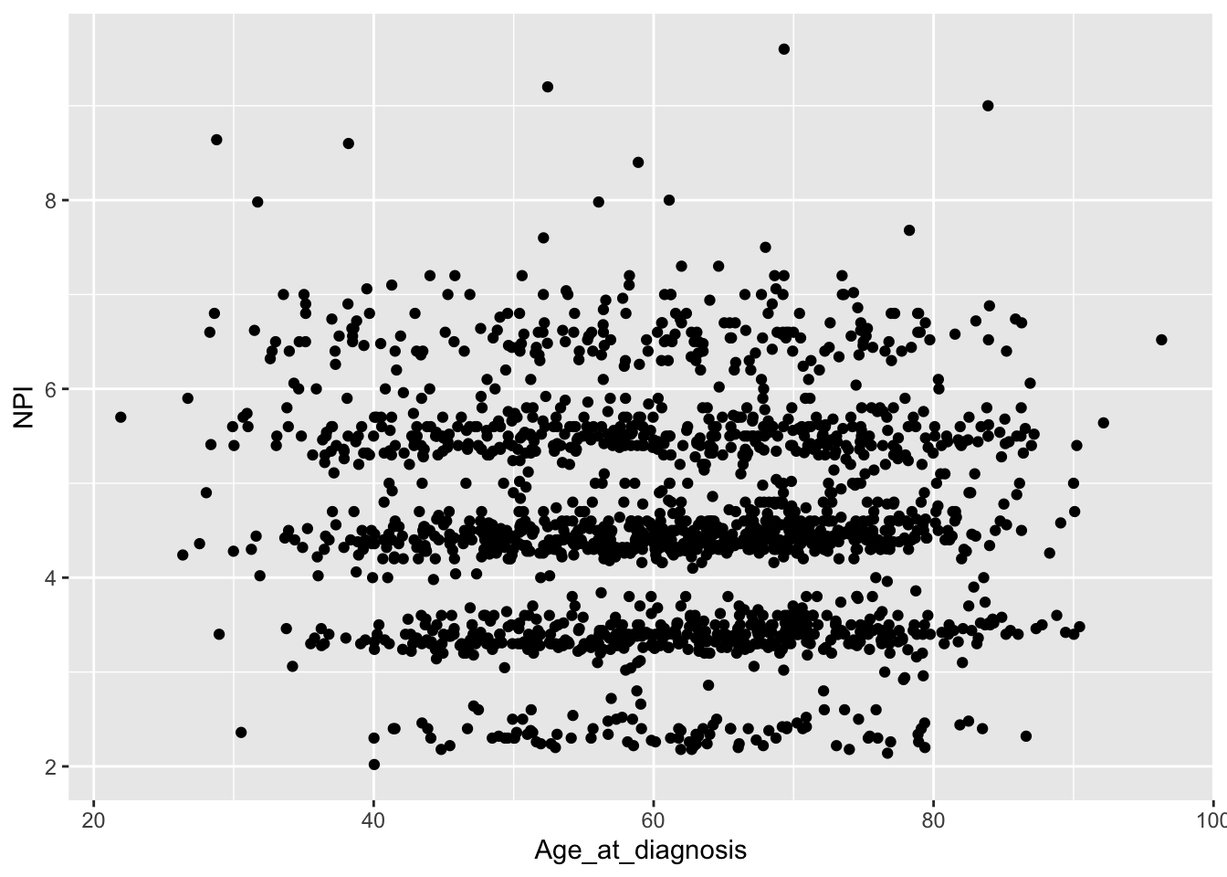
There is still some banding but nothing like the NPI values downloaded from cBioPortal which line up very closely to whole numbers.
The round() function is really useful for rounding numerical values to a specified number of decimal places. We’ll read in the METABRIC data again and create a small workflow that carries out the tumour size conversion, computes the NPI, rounds the tumour size and the resulting NPI value to 1 decimal place and displays the results in decreasing order of NPI.
read_csv("data/metabric_clinical_and_expression_data.csv") %>%
  mutate(Tumour_size = Tumour_size / 10) %>%
  mutate(NPI = 0.2 * Tumour_size + Lymph_node_status + Neoplasm_histologic_grade) %>%
  mutate(Tumour_size = round(Tumour_size, digits = 1)) %>%
  mutate(NPI = round(NPI, digits = 1)) %>%
  arrange(desc(NPI)) %>%
  select(Tumour_size, Lymph_node_status, Neoplasm_histologic_grade, NPI)
## # A tibble: 1,904 x 4
## Tumour_size Lymph_node_status Neoplasm_histologic_grade NPI
## <dbl> <dbl> <dbl> <dbl>
## 1 18 3 3 9.6
## 2 16 3 3 9.2
## 3 15 3 3 9
## 4 13 3 3 8.6
## 5 18.2 2 3 8.6
## 6 12 3 3 8.4
## 7 10 3 3 8
## 8 9.9 3 3 8
## 9 9.9 3 3 8
## 10 8.4 3 3 7.7
## # … with 1,894 more rowsMutating multiple columns
In that last workflow we included the same rounding operation applied to two different variables. It would be nice to be able to carry out just the one mutate() but apply it to both Tumour_size and NPI columns and we can using mutate_at().
metabric %>%
  mutate_at(vars(Tumour_size, NPI), round, digits = 1) %>%
  select(Patient_ID, Tumour_size, NPI)
## # A tibble: 1,904 x 3
## Patient_ID Tumour_size NPI
## <chr> <dbl> <dbl>
## 1 MB-0000 2.2 6.4
## 2 MB-0002 1 4.2
## 3 MB-0005 1.5 4.3
## 4 MB-0006 2.5 4.5
## 5 MB-0008 4 6.8
## 6 MB-0010 3.1 4.6
## 7 MB-0014 1 4.2
## 8 MB-0022 2.9 4.6
## 9 MB-0028 1.6 5.3
## 10 MB-0035 2.8 3.6
## # … with 1,894 more rowsThis is slightly more complicated. We had to group the variables for which we want the function to apply using vars(). We then gave the function name as the next argument and finally any additional arguments that the function needs, in this case the number of digits.
We can use the range operator and the same helper functions as we did for selecting columns using select() inside vars().
For example, we might decide that our expression values are given to a much higher degree of precision than is strictly necessary.
metabric %>%
  mutate_at(vars(ESR1:MLPH), round, digits = 2) %>%
  select(Patient_ID, ESR1:MLPH)
## # A tibble: 1,904 x 9
## Patient_ID ESR1 ERBB2 PGR TP53 PIK3CA GATA3 FOXA1 MLPH
## <chr> <dbl> <dbl> <dbl> <dbl> <dbl> <dbl> <dbl> <dbl>
## 1 MB-0000 8.93 9.33 5.68 6.34 5.7 6.93 7.95 9.73
## 2 MB-0002 10.0 9.73 7.51 6.19 5.76 11.2 11.8 12.5
## 3 MB-0005 10.0 9.73 7.38 6.4 6.75 9.29 11.7 10.3
## 4 MB-0006 10.4 10.3 6.82 6.87 7.22 8.67 11.9 10.5
## 5 MB-0008 11.3 9.96 7.33 6.34 5.82 9.72 11.6 12.2
## 6 MB-0010 11.2 9.74 5.95 5.42 6.12 9.79 12.1 11.4
## 7 MB-0014 10.8 9.28 7.72 5.99 7.48 8.37 11.5 10.8
## 8 MB-0022 10.4 8.61 5.59 6.17 7.59 7.87 10.7 9.95
## 9 MB-0028 12.5 10.7 5.33 6.22 6.25 10.3 12.2 10.9
## 10 MB-0035 7.54 11.5 5.59 6.41 5.99 10.2 12.8 13.5
## # … with 1,894 more rowsOr we could decide that all the columns whose names end with “_status" are in fact categorical variables and should be converted to factors.
metabric %>%
  mutate_at(vars(ends_with("_status")), as.factor) %>%
  select(Patient_ID, ends_with("_status"))
## # A tibble: 1,904 x 7
## Patient_ID Survival_status Vital_status Lymph_node_stat… ER_status
## <chr> <fct> <fct> <fct> <fct>
## 1 MB-0000 LIVING Living 3 Positive
## 2 MB-0002 LIVING Living 1 Positive
## 3 MB-0005 DECEASED Died of Dis… 2 Positive
## 4 MB-0006 LIVING Living 2 Positive
## 5 MB-0008 DECEASED Died of Dis… 3 Positive
## 6 MB-0010 DECEASED Died of Dis… 1 Positive
## 7 MB-0014 LIVING Living 2 Positive
## 8 MB-0022 DECEASED Died of Oth… 2 Positive
## 9 MB-0028 DECEASED Died of Oth… 2 Positive
## 10 MB-0035 DECEASED Died of Dis… 1 Positive
## # … with 1,894 more rows, and 2 more variables: PR_status <fct>,
## # HER2_status <fct>Anonymous functions
The mutate_at() function, and the related mutate_if() and mutate_all() functions, are really very powerful but with that comes additional complexity.
For example, we may come across situations where we’d like to apply the same operation to multiple columns but where there is no available function in R to do what we want.
Let’s say we want to convert the petal and sepal measurements in the iris data set from centimetres to millimetres. We’d either need to create a new function to do this conversion or we could use what is known as an anonymous function, also known as a lambda expression.
There is no ‘multiply by 10’ function and it seems a bit pointless to create one just for this conversion so we’ll use an anonymous function instead – anonymous because it has no name, it’s an in situ function only used in our mutate_at() function call.
iris %>%
  as_tibble() %>%
  mutate_at(vars(Sepal.Length:Petal.Width), ~ . * 10)
## # A tibble: 150 x 5
## Sepal.Length Sepal.Width Petal.Length Petal.Width Species
## <dbl> <dbl> <dbl> <dbl> <fct>
## 1 51 35 14 2 setosa
## 2 49 30 14 2 setosa
## 3 47 32 13 2 setosa
## 4 46 31 15 2 setosa
## 5 50 36 14 2 setosa
## 6 54 39 17 4 setosa
## 7 46 34 14 3 setosa
## 8 50 34 15 2 setosa
## 9 44 29 14 2 setosa
## 10 49 31 15 1 setosa
## # … with 140 more rowsThe ~ denotes that we’re using an anonymous function (it is the symbol for formulae in R) and the . is a placeholder for the column being operated on. In this case, we’re multiplying each of the columns between Sepal.Length and Petal.Width inclusive by 10.
If you think this is getting fairly complicated you’d be right. We’ll leave it there for now but point you to the help page for mutate_at if you’re interested in finding out more.
Computing summary values using summarise()
We’ll cover the fifth of the main dplyr ‘verb’ functions, summarise(), only briefly here. This function computes summary values for one or more variables (columns) in a table. Here we will summarise values for the entire table but this function is much more useful in combination with group_by() in working on groups of observations within the data set. We will look at summarizing groups of observations next week.
Any function that calculates a single scalar value from a vector can be used with summarise(). For example, the mean() function calculates the arithmetic mean of a numeric vector. Let’s calculate the average ESR1 expression for tumour samples in the METABRIC data set.
mean(metabric$ESR1)## [1] 9.607824The equivalent operation using summarise() is:
summarise(metabric, mean(ESR1))## # A tibble: 1 x 1
## `mean(ESR1)`
## <dbl>
## 1 9.61If you prefer Oxford spelling, in which -ize is preferred to -ise, you’re in luck as dplyr accommodates the alternative spelling.
Both of the above statements gave the same average expression value but these were output in differing formats. The mean() function collapses a vector to single scalar value, which as we know is in fact a vector of length 1. The summarise() function, as with most tidyverse functions, returns another data frame, albeit one in which there is a single row and a single column.
Returning a data frame might be quite useful, particularly if we’re summarising multiple columns or using more than one function, for example computing the average and standard deviation.
summarise(metabric, ESR1_mean = mean(ESR1), ESR1_sd = sd(ESR1))## # A tibble: 1 x 2
## ESR1_mean ESR1_sd
## <dbl> <dbl>
## 1 9.61 2.13Notice how we also named the output columns in this last example.
summarise()
summarise() collapses a data frame into a single row by calculating summary values of one or more of the columns.
It can take any function that takes a vector of values and returns a single value. Some of the more useful functions include:
-
Centre:
mean(),median() -
Spread:
sd(),mad() -
Range:
min(),max(),quantile() -
Position:
first(),last() -
Count:
n()
Note the first(), last() and n() are only really useful when working on groups of observations using group_by().
n() is a special function that returns the number of observations; it doesn’t take a vector argument, i.e. a column.
It is also possible to summarise using a function that takes more than one value, i.e. from multiple columns. For example, we could compute the correlation between the expression of FOXA1 and MLPH.
summarise(metabric, correlation = cor(FOXA1, MLPH))## # A tibble: 1 x 1
## correlation
## <dbl>
## 1 0.898Summarizing multiple columns
Much like mutate() with its mutate_at(), mutate_if() and mutate_all() variants, there is a family of summarise() functions similarly named for applying the same summarization function to multiple columns in a single operation. These work in much the same way as their mutate cousins.
summarise_at() allows us to select the columns on which to operate using an additional vars() argument.
summarise_at(metabric, vars(FOXA1, MLPH), mean)## # A tibble: 1 x 2
## FOXA1 MLPH
## <dbl> <dbl>
## 1 10.8 11.4Selecting the columns is done in the same way as for mutate_at() and select().
summarise_all() summarises values in all columns.
metabric %>%
  select(ESR1:MLPH) %>%
  summarise_all(mean)
## # A tibble: 1 x 8
## ESR1 ERBB2 PGR TP53 PIK3CA GATA3 FOXA1 MLPH
## <dbl> <dbl> <dbl> <dbl> <dbl> <dbl> <dbl> <dbl>
## 1 9.61 10.8 6.24 6.20 5.97 9.50 10.8 11.4You have to be careful with summarise_all() that all columns can be summarised with the given summary function. For example, what happens if we try to compute an average of a set of character values?
summarise_all(metabric, mean, na.rm = TRUE)## Warning in mean.default(Patient_ID, na.rm = TRUE): argument is not numeric
## or logical: returning NA## Warning in mean.default(Survival_status, na.rm = TRUE): argument is not
## numeric or logical: returning NA## Warning in mean.default(Vital_status, na.rm = TRUE): argument is not
## numeric or logical: returning NA## Warning in mean.default(Chemotherapy, na.rm = TRUE): argument is not
## numeric or logical: returning NA## Warning in mean.default(Radiotherapy, na.rm = TRUE): argument is not
## numeric or logical: returning NA## Warning in mean.default(Cancer_type, na.rm = TRUE): argument is not numeric
## or logical: returning NA## Warning in mean.default(ER_status, na.rm = TRUE): argument is not numeric
## or logical: returning NA## Warning in mean.default(PR_status, na.rm = TRUE): argument is not numeric
## or logical: returning NA## Warning in mean.default(HER2_status, na.rm = TRUE): argument is not numeric
## or logical: returning NA## Warning in mean.default(HER2_status_measured_by_SNP6, na.rm = TRUE):
## argument is not numeric or logical: returning NA## Warning in mean.default(PAM50, na.rm = TRUE): argument is not numeric or
## logical: returning NA## Warning in mean.default(`3-gene_classifier`, na.rm = TRUE): argument is not
## numeric or logical: returning NA## Warning in mean.default(Cellularity, na.rm = TRUE): argument is not numeric
## or logical: returning NA## Warning in mean.default(Integrative_cluster, na.rm = TRUE): argument is not
## numeric or logical: returning NA## # A tibble: 1 x 34
## Patient_ID Cohort Age_at_diagnosis Survival_time Survival_status
## <dbl> <dbl> <dbl> <dbl> <dbl>
## 1 NA 2.64 61.1 125. NA
## # … with 29 more variables: Vital_status <dbl>, Chemotherapy <dbl>,
## # Radiotherapy <dbl>, Tumour_size <dbl>, Tumour_stage <dbl>,
## # Neoplasm_histologic_grade <dbl>, Lymph_nodes_examined_positive <dbl>,
## # Lymph_node_status <dbl>, Cancer_type <dbl>, ER_status <dbl>,
## # PR_status <dbl>, HER2_status <dbl>,
## # HER2_status_measured_by_SNP6 <dbl>, PAM50 <dbl>,
## # `3-gene_classifier` <dbl>, Nottingham_prognostic_index <dbl>,
## # Cellularity <dbl>, Integrative_cluster <dbl>, Mutation_count <dbl>,
## # ESR1 <dbl>, ERBB2 <dbl>, PGR <dbl>, TP53 <dbl>, PIK3CA <dbl>,
## # GATA3 <dbl>, FOXA1 <dbl>, MLPH <dbl>, Deceased <dbl>, NPI <dbl>We get a lot of warning messages and NA values for those columns for which computing an average does not make sense.
summarise_if() can be used to select those values for which a summarization function is appropriate.
summarise_if(metabric, is.numeric, mean, na.rm = TRUE)## # A tibble: 1 x 19
## Cohort Age_at_diagnosis Survival_time Tumour_size Tumour_stage
## <dbl> <dbl> <dbl> <dbl> <dbl>
## 1 2.64 61.1 125. 2.62 1.75
## # … with 14 more variables: Neoplasm_histologic_grade <dbl>,
## # Lymph_nodes_examined_positive <dbl>, Lymph_node_status <dbl>,
## # Nottingham_prognostic_index <dbl>, Mutation_count <dbl>, ESR1 <dbl>,
## # ERBB2 <dbl>, PGR <dbl>, TP53 <dbl>, PIK3CA <dbl>, GATA3 <dbl>,
## # FOXA1 <dbl>, MLPH <dbl>, NPI <dbl>It is possible to summarise using more than one function in which case a list of functions needs to be provided.
summarise_at(metabric, vars(ESR1, ERBB2, PGR), list(mean, sd))## # A tibble: 1 x 6
## ESR1_fn1 ERBB2_fn1 PGR_fn1 ESR1_fn2 ERBB2_fn2 PGR_fn2
## <dbl> <dbl> <dbl> <dbl> <dbl> <dbl>
## 1 9.61 10.8 6.24 2.13 1.36 1.02Pretty neat but I’m not sure about those column headings in the output – fortunately we have some control over these.
summarise_at(metabric, vars(ESR1, ERBB2, PGR), list(average = mean, stdev = sd))## # A tibble: 1 x 6
## ESR1_average ERBB2_average PGR_average ESR1_stdev ERBB2_stdev PGR_stdev
## <dbl> <dbl> <dbl> <dbl> <dbl> <dbl>
## 1 9.61 10.8 6.24 2.13 1.36 1.02Anonymous functions
The mutate_ functions and summarise_ functions work in a very similar manner, very much in line with the coherent and consistent framework provided by dplyr and the entire tidyverse. For example, we could use an anonymous function in a summarise_at() operation applied to multiple variables. In the assignment from last week, we asked you to compute the correlation of the expression for FOXA1 against all other genes to see which was most strongly correlated. Here is how we could do this in a single summarise_at() statement using an anonymous function.
summarise_at(metabric, vars(ESR1:MLPH, -FOXA1), ~ cor(., FOXA1))## # A tibble: 1 x 7
## ESR1 ERBB2 PGR TP53 PIK3CA GATA3 MLPH
## <dbl> <dbl> <dbl> <dbl> <dbl> <dbl> <dbl>
## 1 0.724 0.280 0.390 -0.0700 -0.149 0.781 0.898Notice how we selected all genes between ESR1, the first gene column in our data frame, and MLPH, the last gene column, but then excluded FOXA1 as we’re not all that interested in the correlation of FOXA1 with itself (we know the answer is 1).
Faceting with ggplot2
Finally, let’s change tack completely and take a look at a very useful feature of ggplot2 – faceting.
Faceting allows you to split your plot into subplots, or facets, based on one or more categorical variables. Each of the subplots displays a subset of the data.
There are two faceting functions, facet_wrap() and facet_grid().
Let’s create a scatter plot of GATA3 and ESR1 expression values where we’re displaying the PR positive and PR negative patients using different colours. This is a very similar to a plot we created last week.
ggplot(data = metabric, mapping = aes(x = GATA3, y = ESR1, colour = PR_status)) +
  geom_point(size = 0.5, alpha = 0.5)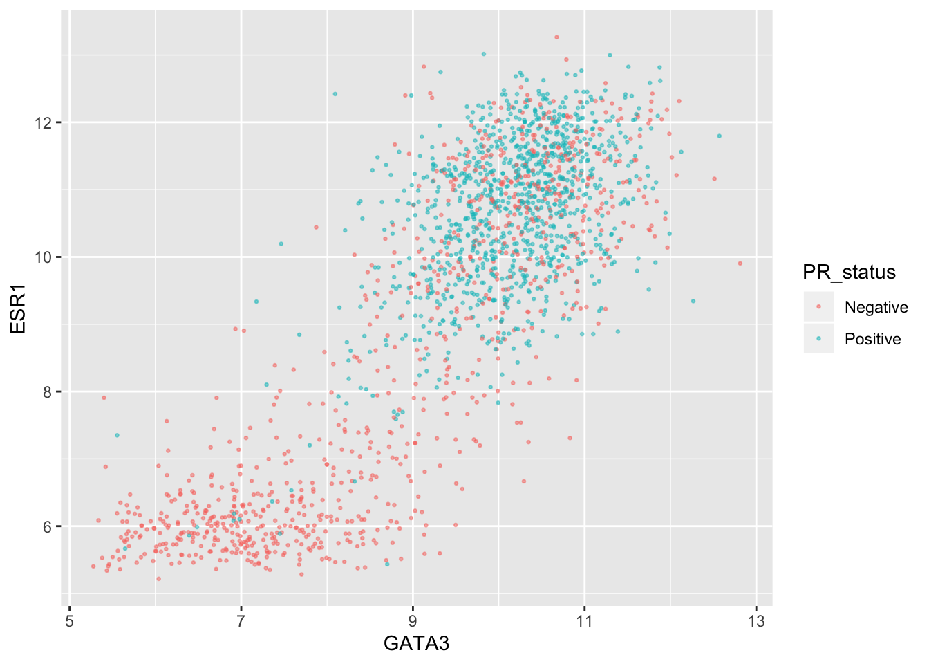
An alternative is to use faceting with facet_wrap().
ggplot(data = metabric, mapping = aes(x = GATA3, y = ESR1)) +
  geom_point(size = 0.5, alpha = 0.5) +
  facet_wrap(vars(PR_status))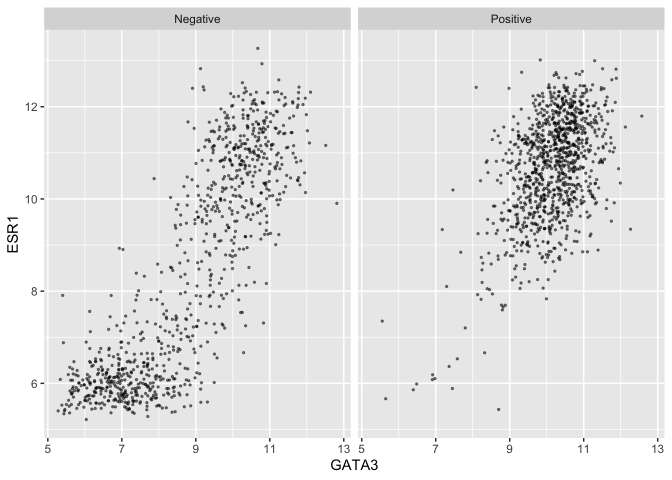
This produces two plots, side-by-side, one for each of the categories in the PR_status variable, with a banner across the top of each for the category.
The variable(s) used for faceting are specified using vars() in a similar way to the selection of variables for mutate_at() and summarise_at().
We can still use separate colours if we prefer things to be, well, colourful.
ggplot(data = metabric, mapping = aes(x = GATA3, y = ESR1, colour = PR_status)) +
  geom_point(size = 0.5, alpha = 0.5) +
  facet_wrap(vars(PR_status))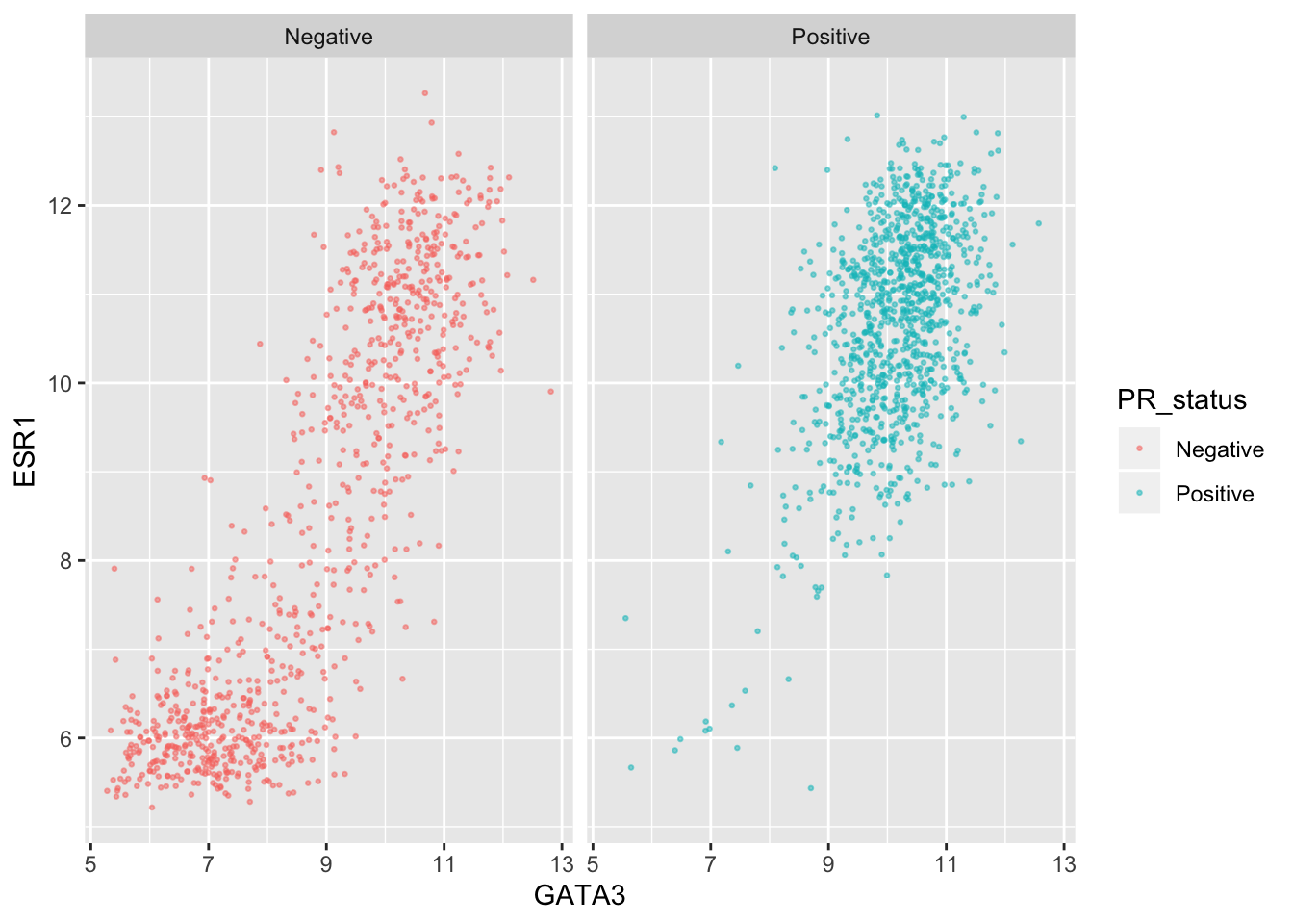
Faceting is usually better than displaying groups using different colours when there are more than two or three groups when it can be difficult to really tell which points belong to each group. A case in point is for the 3-gene classification in the GATA3 vs ESR1 scatter plot we created last week. Let’s create a faceted version of that plot.
ggplot(data = metabric, mapping = aes(x = GATA3, y = ESR1, colour = `3-gene_classifier`)) +
  geom_point(size = 0.5, alpha = 0.5) +
  facet_wrap(vars(`3-gene_classifier`))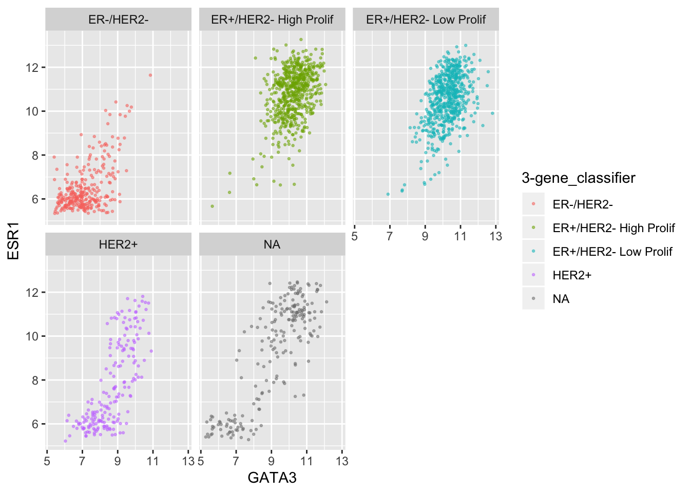
This helps explain why the function is called facet_wrap(). When it has too many subplots to fit across the page, it wraps around to another row. We can control how many rows or columns to use with the nrow and ncol arguments.
ggplot(data = metabric, mapping = aes(x = GATA3, y = ESR1, colour = `3-gene_classifier`)) +
  geom_point(size = 0.5, alpha = 0.5) +
  facet_wrap(vars(`3-gene_classifier`), nrow = 1)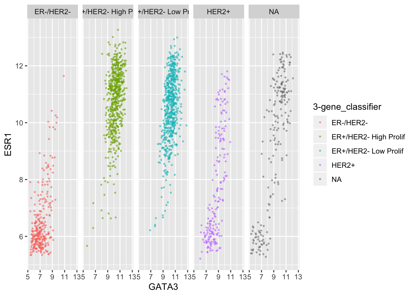
ggplot(data = metabric, mapping = aes(x = GATA3, y = ESR1, colour = `3-gene_classifier`)) +
  geom_point(size = 0.5, alpha = 0.5) +
  facet_wrap(vars(`3-gene_classifier`), ncol = 2)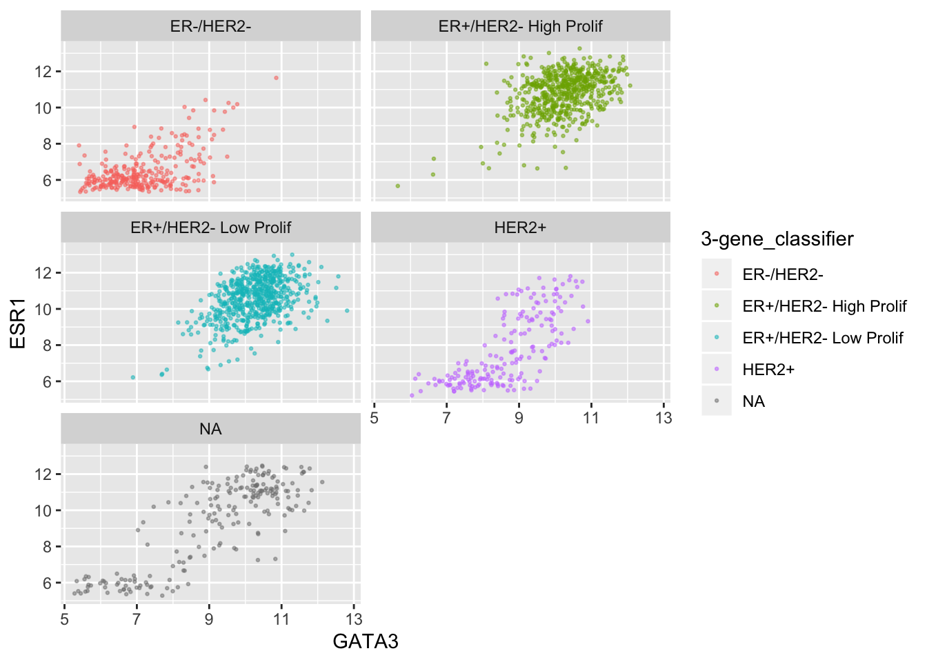
We can combine faceting on one variable with a colour aesthetic for another variable. For example, let’s show the tumour stage status using faceting and the HER2 status using colours.
ggplot(data = metabric, mapping = aes(x = GATA3, y = ESR1, colour = HER2_status)) +
  geom_point(size = 0.5, alpha = 0.5) +
  facet_wrap(vars(Neoplasm_histologic_grade))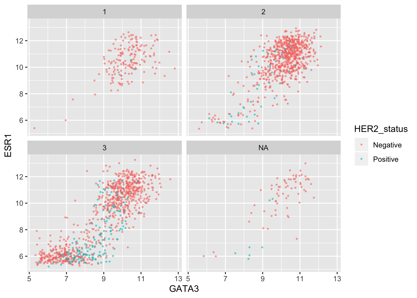
Instead of this we could facet on more than variable.
ggplot(data = metabric, mapping = aes(x = GATA3, y = ESR1)) +
  geom_point(size = 0.5, alpha = 0.5) +
  facet_wrap(vars(Neoplasm_histologic_grade, HER2_status))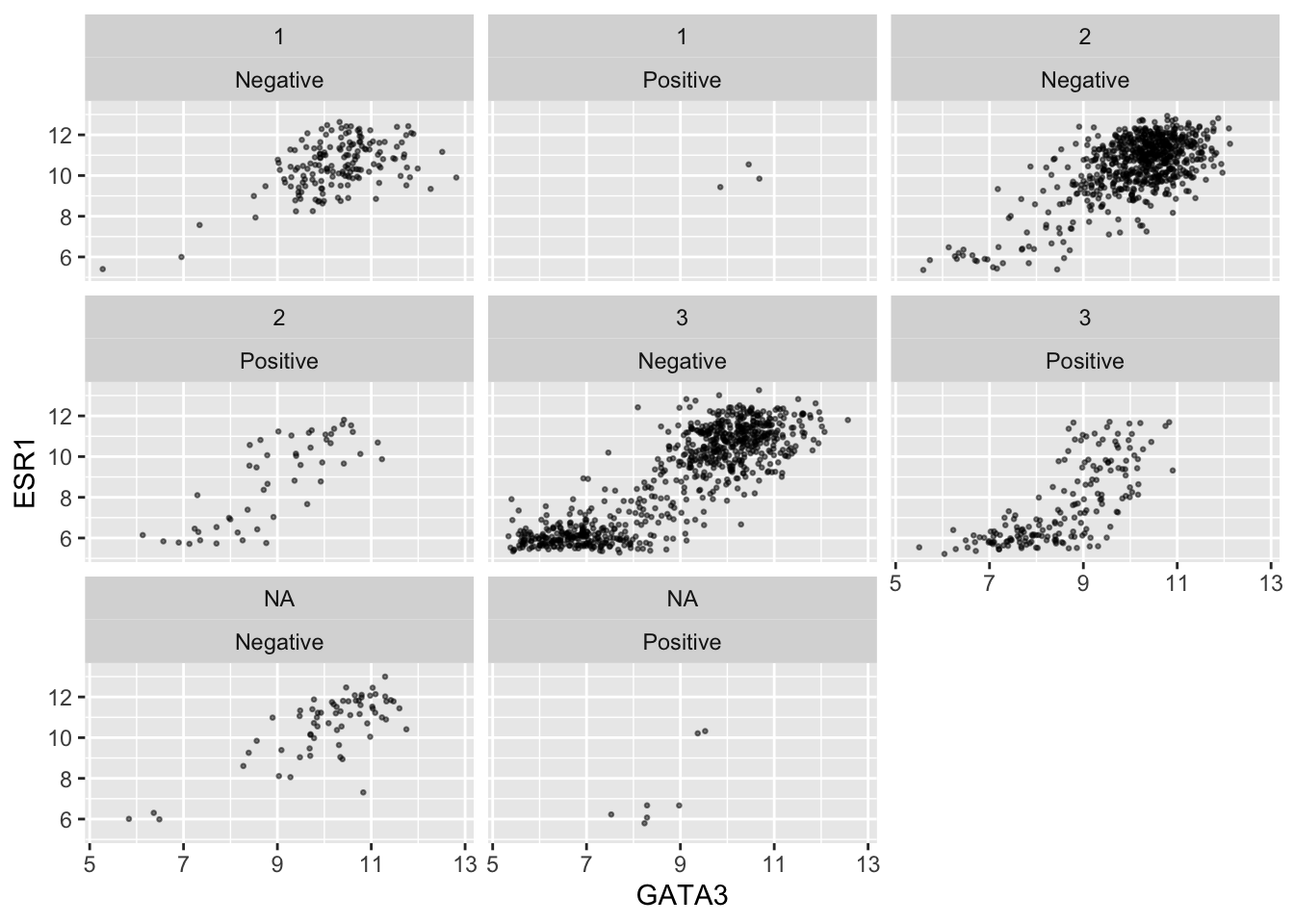
Faceting on two variables is usually better done using the other faceting function, facet_grid(). Note the change in how the formula is written.
ggplot(data = metabric, mapping = aes(x = GATA3, y = ESR1)) +
  geom_point(size = 0.5, alpha = 0.5) +
  facet_grid(vars(Neoplasm_histologic_grade), vars(HER2_status))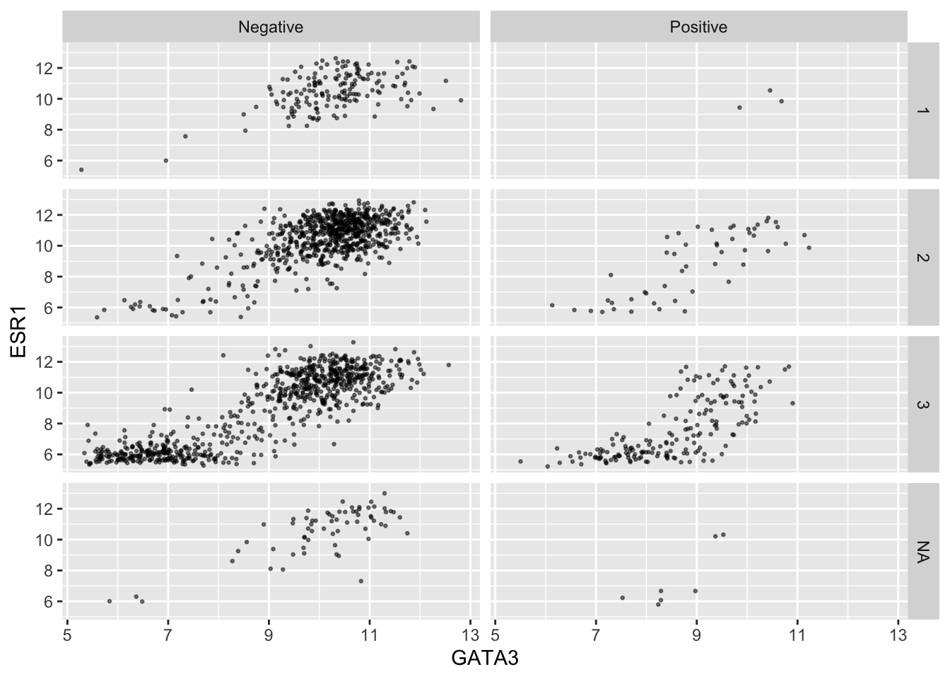
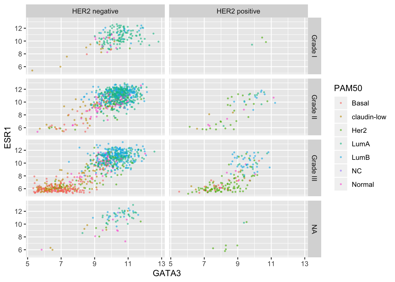
Again we can use colour aesthetics alongside faceting to add further information to our visualization.
ggplot(data = metabric, mapping = aes(x = GATA3, y = ESR1, colour = PAM50)) +
  geom_point(size = 0.5, alpha = 0.5) +
  facet_grid(vars(Neoplasm_histologic_grade), vars(HER2_status))
Finally, we can use a labeller to change the labels for each of the categorical values so that these are more meaningful in the context of this plot.
grade_labels <- c("1" = "Grade I", "2" = "Grade II", "3" = "Grade III")
her2_status_labels <- c("Positive" = "HER2 positive", "Negative" = "HER2 negative")
#
ggplot(data = metabric, mapping = aes(x = GATA3, y = ESR1, colour = PAM50)) +
  geom_point(size = 0.5, alpha = 0.5) +
  facet_grid(vars(Neoplasm_histologic_grade),
             vars(HER2_status),
             labeller = labeller(
               Neoplasm_histologic_grade = grade_labels,
               HER2_status = her2_status_labels
              )
            )
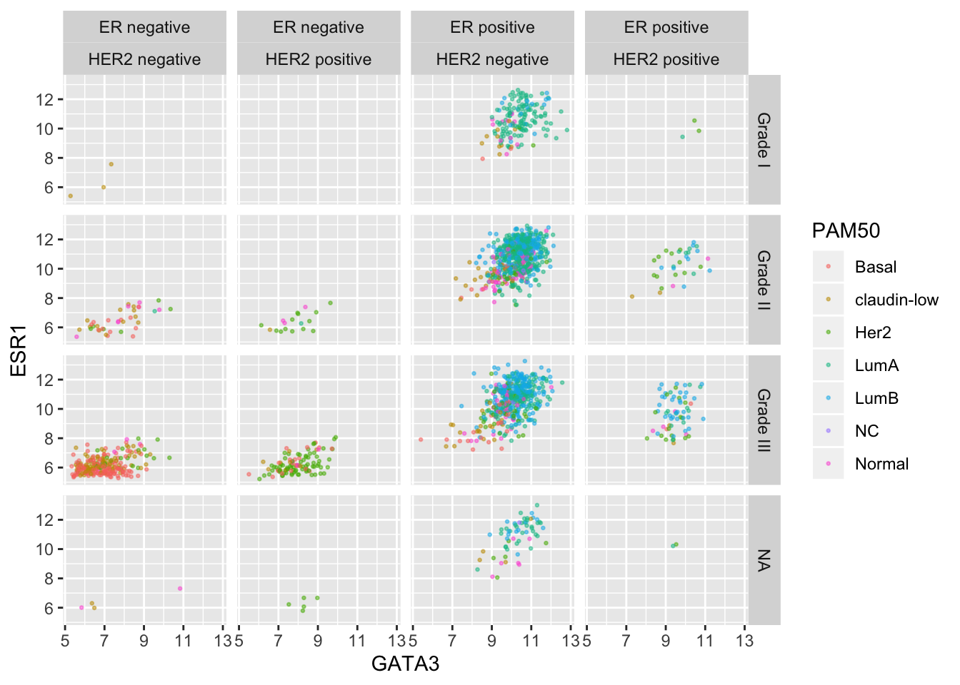
This would certainly be necessary if we were to use ER and HER2 status on one side of the grid.
er_status_labels <- c("Positive" = "ER positive", "Negative" = "ER negative")
#
ggplot(data = metabric, mapping = aes(x = GATA3, y = ESR1, colour = PAM50)) +
  geom_point(size = 0.5, alpha = 0.5) +
  facet_grid(vars(Neoplasm_histologic_grade),
             vars(ER_status, HER2_status),
             labeller = labeller(
               Neoplasm_histologic_grade = grade_labels,
               ER_status = er_status_labels,
               HER2_status = her2_status_labels
              )
            )
Summary
In this session we have covered the following concepts:
- Filtering rows in a data frame based on their values
- Selecting and reordering of columns
- Sorting rows based on values in one or more columns
- Modifying a data frame by either adding new columns or modifying existing ones
- Summarizing the values in one or more columns
- Building up workflows by chaining operations together using the pipe operator
- Faceting of ggplot2 visualizations
Assignment
Assignment: assignment4.Rmd
Solutions: assignment4_solutions.Rmd and assignment4_solutions.html