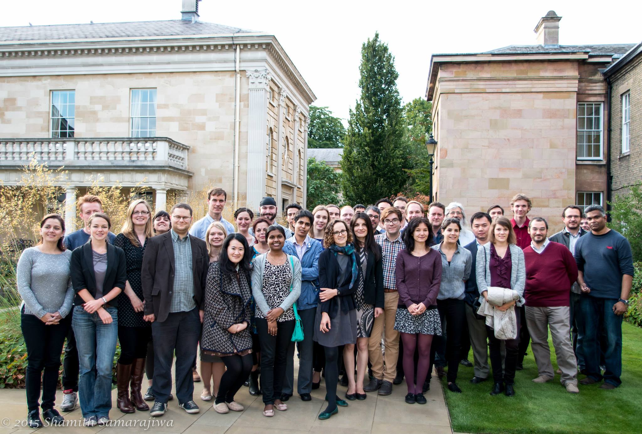
Description.

High-throughput technologies such as next generation sequencing (NGS) can routinely produce massive amounts of data. These technologies allow us to describe all variants in a genome or to detect the whole set of transcripts that are present in a cell or tissue. However, such datasets pose new challenges in the way the data have to be analyzed, annotated and interpreted which are not trivial and are daunting to the wet-lab biologist. This course covers state-of-the-art and best-practice tools for NGS RNA-seq and ChIP-seq data analysis, which are of major relevance in today’s genomic and gene expression studies.

Instructors.

  • Mark Dunning
  • Bernard Pereira
  • Oscar Rueda
  • Ines De Santiago
  • Shamith Samarajiwa
  • Prerequisites.

    There is a lot of material to cover in the course, so we will assume that you are familiar with a few basics before you come. The tool that will we do most of the analysis in is R. There will be a short recap of the key concepts at the beginning of the course; however it will be beneficial if you are already familiar with the following

  • Using the RStudio program
  • Setting your working directory
  • Creating variables and basic object types; in particular vectors and data frames
  • Using built-in R functions
  • Using R to get help on functions
  • Subset operations for vectors and data frames using the [] notation
  • Reading files into R
  • Basic plots; scatter plots, boxplot and histogram
  • Conditional statements using if and else (not essential, but highly recommended)
  • Achieving repetitive tasks using a for loop (not essential, but highly recommended)
  • Several Online videos are available that cover this materials. For example

  • http://shop.oreilly.com/product/0636920034834.do
  • http://blog.revolutionanalytics.com/2012/12/coursera-videos.html
  • http://bitesizebio.com/webinar/20600/beginners-introduction-to-r-statistical-software
  • Or feel free to look through the lecture notes of our University R course Some introductory statistics will be also be assumed. See Statistics at Square One for a good overview.

    Aims.

  • To provide an understanding of how aligned sequencing reads, genome sequences and genomic regions are represented in R.
  • To encourage confidence in reading sequencing reads into R, performing quality assessment and executing standard pipelines for RNA-Seq and ChIP-Seq analysis
  • Objectives.

  • Know what tools are available in Bioconductor for HTS analysis and understand the basic object-types that are utilised.
  • Given a set of gene identifiers, find out whereabouts in the genome they are located, and vice-versa (i.e. go from genomic coordinates to genes).
  • Produce a list of differentially expressed genes from an RNA-Seq experiment.
  • Import a set of ChIP-Seq peaks and investigate their biological context.
  • Course Materials.

    Day One.

  • Introduction to Bioconductor and exploratory data analysis (L) [ Printable PDF ]
  • R and Bioconductor recap (P)
  • Introduction to NGS Sequencing (L) [ Printable PDF ]
  • Quality Assessment of NGS Data (L)
  • Quality Assessment of NGS Data (P)
  • Quality Assessment of NGS Data (Quiz!)
  • Alignment Slides
  • Alignment Demo
  • Day Two.

  • Representing Sequencing data in Bioconductor (L) [ Printable PDF ]
  • Representing Sequencing data in Bioconductor (P)
  • Linear Models and Experimental Design (L)
  • Introduction to RNA Sequencing (L)
  • RNA-Seq counts to reads (P)
  • Day Three.

  • RNA-seq Practical
  • (Supplementary) RNA-seq Practical
  • Introduction to Genome Annotation[ Printable PDF ]
  • Genome Annotation Practical
  • Using Genome Browsers (L)
  • Day Four.

  • Downstream Analysis of RNA-seq Data (L)
  • Downstream Analysis of RNA-seq Data (P)
  • Introduction to ChIP-Seq (L)
  • Analysis of ChIP-Seq (L)
  • ChIP-Seq Practical
  • Reproducible Research[ Printable PDF ]
  • Day Five.

  • Downstream Analysis of ChIP-Seq Data (L)
  • Downstream Analysis of ChIP-Seq Data (P)
  • How to Run the course.

    We recommend using RStudio for the practicals along with R version 3.2.1

    Download the materials from this repository and install the required R and Bioconductor packages from within RStudio. This may take several minutes.

    source("http://www.bioconductor.org/biocLite.R")
    biocLite(c("Biostrings", "ShortRead", "DESeq", "edgeR","biomaRt", "BSgenome",
               "pasillaBamSubset", "pasilla",
               "rtracklayer", "ggbio", "vsn","gplots","RColorBrewer","chipseq","htSeqTools","limma","NBPSeq","tweeDEseqCountData","org.Hs.eg.db","Rcade", "ChIPQC","TxDb.Hsapiens.UCSC.hg19.knownGene","BSgenome.Hsapiens.UCSC.hg19","ChIPpeakAnno","statmod","locfit","Rsubread","goseq","GO.db"))
    
    The Download zip file link at the top of this page will download all the lectures and practicals, and some example data. However, larger data files have to be downloaded from elsewhere because they are too large to share on github

    Example Data.

    Day 1

    A breast cancer dataset is also required for the Bioconductor introductory practical. This folder can be downloaded from Dropbox. Once downloaded and unzipped, the folder should be placed inside the Day1 directory

  • Example chromosome 6 reads
  • Chromosome 6 reference sequence
  • Day 2

  • 1000genomes sample, chromosome 22 aligned reads bam
  • 1000genomes sample, chromosome 22 aligned reads bam index
  • Chromosome 22 reference sequence
  • RNA-seq sample 16N aligned bam
  • RNA-seq sample 16N aligned bam index
  • RNA-seq sample 16T aligned bam
  • RNA-seq sample 16T aligned bam index
  • RNA-seq sample 18N aligned bam
  • RNA-seq sample 18N aligned bam index
  • RNA-seq sample 18T aligned bam
  • RNA-seq sample 18T aligned bam index
  • RNA-seq sample 19N aligned bam
  • RNA-seq sample 19N aligned bam index
  • RNA-seq sample 19T aligned bam
  • RNA-seq sample 19N aligned bam index
  • Using Docker.


    If you not attending one of our courses in-person you can still run the course materials using the Docker system. First, you will need to install the boot2Docker software.

    Once you have boot2docker installed, an icon should appear on your Desktop (Windows) or Applications folder (Mac). After running this new application, a new window should appear will various lines of white text on a black background. The last line should read;

    docker@boot2docker:~$
    Now carefully type the following line of text (using the correct spaces and punctuation is very important!)
    docker run -p 8787:8787 markdunning/cruk-bioinf-sschool
    This will download and install some data. Once this has finished, you can open a web browser and type the following. This will launch a version of RStudio within your browser. You will need to enter the username 'rstudio' and password 'rstudio'.
    http://localhost:8787
    For exercises which use the command-line (e.g. alignment and qa practicals) run the following command in boot2docker
    docker run -ti markdunning/cruk-bioinf-sschool /bin/bash

    License

    This work is licensed under the Creative Commons Attribution-ShareAlike 2.0 UK: England & Wales License. To view a copy of this license, visit http://creativecommons.org/licenses/by-sa/2.0/uk/ or send a letter to Creative Commons, 444 Castro Street, Suite 900, Mountain View, California, 94041, USA.

    Resources
  • seqanswers Bioinformatics forum
  • Biostars forum
  • Bioconductor forum
  • R-bloggers
  • NGS wiki